Chapter Fifteen

THE RESEARCH, DEVELOPMENT AND APPLICATION OF SIGNIFICANT TECHNIQUES

15.1. TRANSMITTERS

15.2. RECEIVERS

15.3. RADAR ANTENNA DESIGN TECHNOLOGY 1949-2009

15.4. CIRCULAR POLARISATION

15.5. M.T.I.

15.6. STRIPLINE

15.7. PULSE COMPRESSION

15.8. THE INTRODUCTION OF DIGITAL AND SOFTWARE PROCESSING IN RADAR SYSTEM

---

15.1. TRANSMITTERS

The years following the Second World War witnessed far-reaching and progressive developments of radar transmitters.

Following its rapid development during the war, the Magnetron remained the primary source of RF power up to a few Megawatts peak until well into the 1950's. Originally a fixed-frequency oscillator, later enhancements enabled a degree of tuning by means of adjustment to its resonant cavities, albeit a relatively slow adjustment. While simple and robust, the magnetron exhibited a tendency to oscillate at other than the desired frequency (mode), which placed constraints on the character of the input pulse applied to it.

The magnetron required a high voltage pulse of power, normally some tens of kilovolts, and of well-defined pulse length and shape. This was typically provided by a ‘Line type’ modulator consisting of a pulse-forming network (lumped delay line - PFN) charged, typically resonantly, from a voltage supply of several hundreds of volts and then discharged via a switch and a step-up pulse transformer into the magnetron. The switch, originally a spark gap in the early days, was normally a hydrogen thyratron. The performance of such a system was limited not only by the magnetron characteristics but also by the characteristics of the PFN, the pulse transformer and the switch. The limitations combined to place constraints on the frequency stability, pulse-rate stability, RF pulse shape and the RF noise performance.

The advent of early power switching semiconductors, while reducing somewhat the size and the power wastage, did little to enhance the overall transmitter performance.

The advances in Moving Target Indication (MTI) were to require greatly improved stability and noise performance that were impossible practically with a magnetron transmitter. The use of a ‘tunable’ magnetron, which could follow the local oscillator frequency, went some way to enhance MTI performance, but frequency control was still only pulse-to-pulse, rather than intra-pulse. Developments at higher powers, typically used in Type 80 and HF 200, led on ultimately to the AR5 product, which succeeded in combining a high power tunable magnetron with advancing MTI technology.

A major advance in capability came with the advent of the switched driven transmitting tube, such as the klystron or, more typically, the Travelling Wave Tube (TWT). The TWT is normally used as an amplifier, as opposed to an oscillator, so that control, even intra-pulse, of its output frequency by applying a low power driving signal became possible, This allowed frequency-sweep patterns to be applied to the output pulse for MTI, Pulse-Compression and clutter-reduction purposes. The other significant factor was that the TWT power could be switched by an internal grid, similar to the radio valves of history, meaning that the PFN system could be replaced by an energy-storage capacitor whose charged voltage could be maintained within close limits. Furthermore, the switching pulse applied to the grid was of much lower power and could relatively easily be controlled in shape, amplitude, pulse length and repetition frequency as demanded by the requirements of the overall radar system. Thus, almost at a stroke, the transmitter ceased to be the overriding limiting factor on the performance of a sophisticated radar system.

Concurrently with the above developments, two other areas of development were taking place, which allowed full advantage to be taken of transmitting tube developments.

One advance was the increasing availability of reliable semiconductor devices, both power devices and stable signal processing devices. The significant power devices were the Thyristor (or silicon controlled rectifier [SCR] as it was initially known) and the high voltage semiconductor rectifier. The immediate effect was to remove the lossy, large and life-limited thermionic devices that had been needed for controlling high powers and for generating high voltages at powers of tens of kilowatts. It became possible to design high-frequency inverters capable of handling up to around 30kw continuously, and which could easily be switched on and off both for power control and in the event of faults. These inverters were typically resonant inverters operating at approximately 25kHz, the high frequency enabling the use of much smaller step-up transformers to provide the high voltage required by the transmitter tube. A particular advantage of combining high frequency inverters and thyristors was that it became possible to switch off the power supply within about 20 microseconds (faster than any fuse could respond) in the event of a fault such as an arc within the TWT. This, combined with a fast-acting Crowbar circuit to dump the stored energy, both protected the TWT from damage, and, importantly, enabled the transmitter rapidly (within one second) to be returned to normal operation. Without this facility, a fault could at least cause a ‘shut-down’ to replace fuses (with the attendant loss of service), and would also seriously stress many other components in the power train.

Smaller power thyristors and other semiconductor power switches, such as Field-Effect Transistors (FETs), greatly facilitated the generation of the switching pulse for the TWT, again giving flexibility in performance and reducing both size and losses.

The improving low power semiconductors enabled much more accurate sensing of the voltages applied to the TWT, making fuller use of the power devices ability to control the output voltages to increasingly tighter tolerances. A later development saw the application of an in-pulse regulator system, which modulated the TWT body voltage, enabling an even tighter control of the TWT operating parameters. Again, the newer technology brought with it significant improvements in reliability and space utilisation.

The second major development involved advances in high voltage high power components such as EHT transformers, and in the management of power circuits operating at these high voltages. The classical approach had been to immerse high voltage components in ‘ transformer oil’, which, while not without its own problems of reliability, weight, flammability and maintenance, was a well tried an understood technology.

An early move from transformer oil was the use of Sulphur -Hexafluoride (SF6) gas as the EHT insulating medium, and this was used in the AWS-5 radar of the 1980's. This radar used a grid-switched Coupled Cavity TWT having a swept frequency RF drive, but much of the rest of the radar transmitter design remained conventional.

The next step with high voltage technology in this context was the development of Encapsulation techniques, in which EHT transformers and other components used Epoxy Resin rather than liquid or gas as the insulating medium. Early efforts in this direction were challenged by the difficulty in avoiding minute voids, or bubbles, in the resin; these would cause local ionisation under the stress of the high voltage and lead to premature breakdown. This known phenomenon was eventually satisfactorily controlled. Plessey engineers played a leading part in this work in conjunction with their suppliers (Southern Transformers and Encapsil).

A parallel activity was the development of a fuller understanding of the surface characteristics required for operation at EHT potentials in order to prevent discharge and breakdown, both in air and in other fluids. Surface hardening and minimum radius requirements were understood and defined.

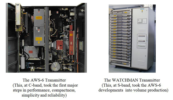
The above advances combined to produce a revolutionary approach to the power-supply side of transmitter design – an all-semiconductor design using encapsulated EHT components along with air-insulation. Volume and weight were reduced and difficult fluids eliminated. The first Plessey design using these principles was the Naval AWS-6 system, which used a C-band TWT capable of 50Kw peak output power.

It is worth noting here that peak output power requirements were now beginning to be reduced as other parts of radar technology advanced. Sophistication was tending to displace ‘brute-force’ power.

The next big step forward in performance, compactness, simplicity and reliability came with the WATCHMAN radar. In this the AWS-6 techniques were refined and applied to an S-band radar. New methods of noise control within the transmitter improved the MTI performance to a level not previously achieved on any ground radar anywhere in the world.

The Watchman transmitter was followed by the type 996 Naval transmitters, in which the same techniques were applied to powering a higher voltage TWT, now in the order of 47Kv. The design well satisfied the on-board requirements for low maintenance, low staffing and minimum training which are essential to the modern warship environment.

The continuing developments in transmitter design, MTI and Pulse Compression performance put the Company's radars in a world-leading position and led to the development of a family of high power land-based radar systems known as the ‘COMMANDER’ range of products, namely AR320, 325 and 327. The higher powers were obtained by employing multiple EHT generation packages running in parallel, taking full advantage of the simplicity and modularity of this type of transmitter design.

By this time Plessey Radar was arguably producing the most reliable and cost effective high power transmitters in the world.

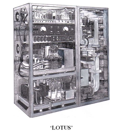
Decca Radar’s first 650Kw, S-Band Transmitter was developed under the LOTUS project in 1956. The prototype was built during the Heavy Radar Laboratory year at Hersham and was ‘productionised’ at Davis Road (Stygals building) on the groups return to Chessington. LOTUS first formed part of the AWS-1 Radar for the Danish Navy in 1957.

In its various forms (only minor modifications) it went on to be manufactured in hundreds, powering AWS-1, DASR-1, LC150, MR100, 43S, WF44, FR-1 and with a ‘Stalo’ fitted for MTI operation was at the centre of the then ‘world leading’ AR-1 RADAR.

LOTUS was improved to deliver some 800Kw of peak power and employed a tunable magnetron and a TWT receiver.

15.2. RADAR RECEIVERS

The receiver is equal in importance to any other element of the Radar System, but it is vulnerable to an unacceptable degree of interfering radiation or deliberate jamming.

The ability to detect and present returned radar signals (echoes) from ‘target’ structures is of paramount importance to both monitor display and integrated signal processing and therefore all possible means of reducing both natural and hostile clutter is continually researched.

Early microwave radar systems had no RF Amplifier, the receiver front end being a waveguide and crystal diode mixer followed by a multi-valve intermediate frequency amplifier. It was therefore essential that the first valve stage of the IF amplifier generated as little noise as possible and had sufficient gain to render following stages unable to add significantly to the receiver noise output.

Early receivers were linear in function with a dynamic range of the order of 30dB maximum. The output of such receivers could easily be saturated with large signals, such as ‘close-in’ ground returns (clutter) or jamming signals, which could render wanted signals, such as aircraft, invisible. (This feature was used in WW2 to hide aircraft within and beyond a high level of clutter signals. This clutter was created by metal foil strips, which were cut to a particular length related to the wavelength of known surveillance/search radars. The strips were dropped by ‘scout aircraft’).

Ground clutter is normally reduced using a simple technique, which reduces the gain of the receiver immediately after the transmitter pulse and gradually allows the gain to increase back to normal full gain. This ‘Swept Gain’ waveform is adjustable in amplitude and length to suit the particular location of the radar.

An early development produced a receiver with a much greater dynamic range, up to some 60-90dB. It had a Logarithmic response i.e. the input/output characteristic is Logarithmic. The Log Receiver utilised a video summing line into which the detected output of each successive amplifier stage was fed. The result produced a rather grey picture on the CRT Display, but was impressively effective in giving a skilled operator visibility of a target in clutter.

The Log Receiver is particularly good when working in conjunction with CP (Circular Polarisation) and the target is in rain.

In 1962 members of the Decca Radar ‘Receiver Design Team’ were briefed at a meeting with SHAPE/SADTC Staff (NATO HQ in the Hague – ‘Air Defence Technical Centre’) on a combination of receiver functions they called CCM2 (Counter, Counter Measures 2). The concept was then adopted by the Decca Radar Company and led to a further development programme from which ECCM Rx’s were incorporated into military radar systems of the time. CCM2 was taken to the market by Decca Radar, as an ECCM RECEIVER package (Electronic Counter, Counter Measures). At this time all receivers were transistorised and were followed at a later date by the use of integrated circuits, which became available from Plessey Caswell.

Along with a Linear and Logarithmic Receiver the Decca Radar ECCM Receiver package comprised a ‘DICKE FIX’ Receiver, a Pulse Length Discriminator (PLD) and an IAGC (Instantaneous Automatic Gain Control) receiver.

A Linear Receiver was always provided to give maximum detection capability in clear conditions. However, experimentation showed that to a skilled operator the Dicke Fix receiver was a close match to the linear receiver.

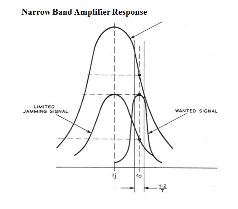
THE DICKE FIX receiver was invented by Professor R. H. Dicke, a citizen of the USA. The basis of his technique is a saturated broadband receiver IF amplifier of a bandwidth some ten times the optimum for the particular radar pulse-length then in use, followed by a final IF stage and detector optimised to the operating system pulse-length. One or two stages of the broadband amplifier needed to be in saturation before the final narrow stage. In CCM2 the Dicke Fix output signal is passed via an adjustable threshold set near the noise level, so that only signals exceeding the threshold are sensed and used to switch the output from the Log/PLD combination to the ECM Receiver output. By the combination of the two channels all ‘out-of-band’ noise (impulse jamming), swept CW adjacent radar interference and non-optimum pulse-length signals are rejected and the operator presented with a display with minimised false alarms. The dynamic range of the Dicke Fix receiver is directly related to the ratio of the inbuilt bandwidths and results in a grey appearance on the radar screen, rather like the plain Log Receiver output. However, it is particularly effective against wide band noise jamming. The CCM2 Receiver Combination gives a quantised output of good contrast and combines the attributes of the component receiver functions.

The PLD Unit (Pulse-length Discriminator) provides the means of processing the output of the Logarithmic Receiver such that only echoes correctly aligned to the transmitted pulse-length are passed to the output.

The IAGC Receiver (Instantaneous Automatic Gain Control) was a further receiver development, having its roots in the collaboration between the Decca Radar Company and SNERI of France, and could be regarded as an alternative to the Log Receiver plus PLD. It was used in a variant of the CCM2/ECCM systems marketed by our Radar Company.

The power supply providing 12volts for the receiver systems was of sophisticated design ensuring stability ‘whatever’ the input, with a no-break facility.

ECCM Receivers, based on the CCM2 concept, aimed to achieve a ‘constant false alarm rate’ (CFAR) in the face of ECM jamming activity, which could include wide band noise or impulse jamming.

Digital processing was in its infancy and detection of a target was very much dependent on a skilled operator seated at a CRT Display. Jamming was effective by desensitising the detection process, also by filling the display with false targets or alarms, making visual detection almost impossible.

Operator confusion was removed by the ECCM/CFAR operation.

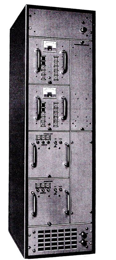
Pre transistorised ECCM circuits would have employed thermionic valves, but later designs followed a progression through discreet silicon transistors to integrated circuit technology, where full IF circuits became available in ‘chip form’ from the Alan Clark (Plessey) Research Establishment at Caswell. The family of radar receivers were subsequently built into all of the Company’s surveillance radars and supplied as update- packages for radars of any manufacture, throughout the world.

The picture shows a typical ECCM Radar Receiver package of R305 type.

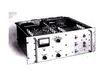
TYPE R405 RADAR RECEIVER

While addressing a similar range of sub-system receiver functions as that of the R305, the R405 took full advantage of developments in component miniaturisation and speed of processing, with the product being marketed against the following parameters:

Wide dynamic range. Good constant false alarm rate. Fast transient signal recovery time. Long-term stability and reliability. Compatible with most air defence and naval radars and provides high-level protection against a variety of jamming signals.

GENERAL

The Type 405 multi-purpose anti-jamming radar receiver embodied the products of modern technology to ensure rejection of received signals whose characteristics did not closely approximate to those of the transmitted pulse (See also the EW section 14.1). The sensitivity of a radar receiver is limited by unwanted signals present at its input. Thermal noise sets an absolute threshold and, in practice, of unwanted signals such as clutter that may also be present. Further interfering signals may be received from adjacent radar, electrical equipment or from hostile jamming sources.

The Type R405 Receiver, in addition to being designed to minimise the effects of interfering signals, provided all the important essentials of a modern radar receiver, including:

• A wide dynamic range, to avoid loss of signal due to saturation.
• Good Constant FAR (False Alarm Rate) performance.
• Fast recovery from large transient signals.
• Long-term stability and reliability avoiding repeat retuning or setting-up.
• Good rejection of jamming signals, resulting in the detection of a ‘self-screening’ target.

The Type R405 had successfully undergone both laboratory and field tests against many forms of electronic counter measures and had facilities ‘built-in’ allowing separation of up to 1000 metres between the Rx and the operators Remote Control Unit.
The R405 was designed to be easily added to existing radars whether or not they were fitted with MTI, Frequency Agility or Automatic Plot Extraction and compatible with all types of pulsed radar having pulse lengths in the range 0.8 to 10µs and operating at an intermediate frequency of 30MHz.

The dual R405 receiver version was configured into a single rack for use with a 2-Beam Radar, or radars with dual transmitters operating in diversity.

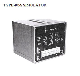
This product was designed to provide, at low cost, various types of ECM training, inclusive of selectable simulated jamming signals. It also enabled testing of the efficiency of operational radar’s ECCM capabilities. It would inject simulated ECM signals at operational radar IF frequencies. (Between 25 and 35 MHz). As a small lightweight unit it was easily added to any operational radar. Outputs from the 405S would include – wideband noise with a bandwith of 60MHz and an IF signal that could be modulated by one or more internally generated waveforms.

TYPE R505 RADAR RECEIVER

This product was again brought to the market with a similar range of functions as that of its predecessors but it was ‘of its time’ in terms of component utilisation, compactness, reliability, accessibility, maintainability and speed of processing of the received signal information. (See also the EW section 14.1)

It was the product of extensive laboratory and field trials against many forms of electronic counter measures, ensuring rejection of all received signals whose characteristics did not closely approximate to those of the transmitted pulse.

It was designed to be easily added to, or included in new ground radar equipments, compatible with all types of pulsed radars having a pulse length of 0.2s to 1.5s operating at an IF of 60MHz. Converter units would be provided for operation at other intermediate frequencies and a pre-amplifier of adequate bandwith (greater than 12 times the optimum for the pulse length of the radar) with a good resistance to saturation and paralysis effect was necessary. If the existing receiver unit fitted did not meet the requirement then a Plessey version could be supplied.

CHARACTERISTICS OF ECCM RECEIVERS THAT RELATE TO EW JAMMING

The combined logical receiver mode comprises the good anti-clutter properties of the log receiver with the protection against jamming signals of the wrong pulse length or frequency (provided respectively by the Pulse Length Discriminator (PLD) and the Dicke-fix receiver). The most effective receiver characteristics for particular forms of electronic interference are as follows:

INTERFERENCE	EFFECTIVE RECEIVER MODE
CW on frequency	Log with PLD.
CW just off frequency	Log with PLD; or Dicke-fix
Long pulse on frequency	Log with PLD.
Short pulse on frequency	Log with PLD; or Dicke-fix
All pulses just off frequency	Dicke-fix
CW swept at any rate	Combined 1ogical receiver
Chaff jamming (Window)	Log with PLD.

15.3. RADAR ANTENNA DESIGN TECHNOLOGY 1949-2009

"The discipline of Microwave Engineering is 10% Mathematical and 90% Black Magic"
Dr. Ken Milne.

REFLECTOR ANTENNAS

As this chapter tracks the history of radar antenna design within the Decca Radar company, the references to the microwave bands are the definitions that existed in those far-off heady days. The reader must research the modern nomenclatures should they not be conversant with them.

PARABOLIC SECTIONS

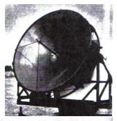
From the earliest days of the Decca Company (formed in the 1940’s) until the 1980’s, most of the antennas were reflectors using either a ‘point’ feed or a line feed as the illuminating source. The reflectors were invariably of parabolic sections. Some reflectors, such as the early X-band wind-finder radars (WF I, II and III), were parabolae of revolution providing a circular dish, some 3m in diameter, always producing a ‘pencil’ beam.

There are other configurations of parabolic reflectors, which are cut sections of a parabola of revolution, cut in such a way as to result in an ‘orange peel’ shaped reflector. These have all the attributes of a parabola of revolution i.e. it is truly parabolic in all planes, except that it produces a ‘fan’ shaped beam. The ratio of azimuth beam to elevation beam will be proportional to the aspect ratio of the reflector. 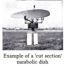Classic examples of an orange peel reflector are the Decca 424 airfield radar, the HF200 and the LC 150. The latter two high power radars being fondly known as ‘Noddy’ and ‘Big-Ears’. The reason for the ‘orange peel look’ is that the edge profile is cut round a line of equal power level typically -10dB with respect to the maximum radiation from the horn feed. This power ‘taper’, or distribution, is the factor that determines the level of sidelobe radiation that the antenna will provide. For an edge taper of -10dB, the sidelobe levels of this type of antenna will be lower than -25dB with respect to the maximum antenna gain.

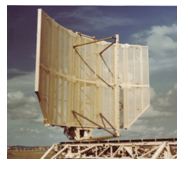A third configuration is a parabolic cylinder, which, as its title suggests, is parabolic in one plane whilst being cylindrical (or linear) in the orthogonal plane. The linear section may be horizontal or vertical depending on the operational requirement. There is no beam shaping from the reflector in the linear (or cylindrical) plane and therefore the radiated beam shape will be a function of the feed. The AR3D antenna shown has its linear dimension vertical and the elevation radiation pattern is that of the line feed.

As described elsewhere (Chapter 7.5; AR3D), this antenna provides electronic beam scanning in the vertical plane and although frequency scanned arrays existed at that time, the technology used in the AR3D design was newly developed by Plessey Radar engineers at Cowes. The AR3D feed uses corrugated waveguide, the design of which, as said, was wholly a product the microwave design group at Cowes. Before describing this it may be helpful to recap the mechanism of beam squint that results from an end fed linear array.

GROUP DELAY IN WAVEGUIDE

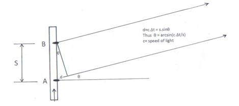
This is a measure of how long a microwave signal takes to pass between two points, say, A and B, in the waveguide. If there are radiating elements at A and B then a signal arriving at A will begin to radiate a portion of the incident signal. Due to the group delay the residue of this signal will reach the element at B at some time Dt (the Group-Delay) later, where-upon element B will radiate. The figure below shows how these signals come into phase to form a beam at angle q with respect to the array normal. Group Delay is a function of frequency for a given waveguide configuration; hence for a change in frequency (Df), with all other things being equal, there will be a corresponding change in Group Delay (Dt) and therefore a change in q, i.e. a BEAM SQUINT.

To achieve a given beam scan sensitivity in say, degrees per megahertz, the waveguide parameters have to be carefully chosen. The usual practice is to use standard waveguide operating in the dominant mode and this means the distance through the waveguide must exceed the physical spacing between the radiating elements, which, for other reasons, cannot be allowed to exceed a given dimension (usually about 0.6 of the free space wavelength). This means that to achieve the desired group delay using standard waveguide the guide must be folded a number of times to increase its electrical length. This results in a ‘serpentine’ (or snake like) feed. Traditionally a serpentine is made up of many ‘U’ bends of waveguide soldered together to form a continuous linear array (unfolded the actual length would be much greater than that of the folded array and carries with it considerable weight and manufacturing disadvantages). The new corrugated feed, used in place of the serpentine, utilised two innovative methods one exploiting a principle of microwave engineering and the other of manufacturing.

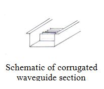The theory relating to the microwave design of a corrugated feed was developed (in house) at Cowes, as was the means by which size, weight and manufacturing difficulties of the serpentine were overcome. The desired Group Delay for beam shaping was obtained by the form and depth of the corrugations and width of the waveguide and could be achieved within the spacing of the radiating elements i.e. there was no need to fold the waveguide. The new waveguide configuration was most amenable to the automated manufacturing techniques of electro-forming and numerically controlled machining, thus providing greater precision and a less labour intensive manufacturing process.

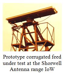Although the corrugated feed was an elegant solution and produced significant benefits, its manufacturing process demanded that it be formed as an open ‘U’ section (see schematic above) meaning that to complete the waveguide it needed a lid. This was a potential problem because the joint at the lid/waveguide interface was at a high current density position and if the joint was in any way less than perfect it would be prone to high power breakdown or microwave leakage. Industrial Engineers at Cowes took on this challenge and adopted a process known as ‘Electron Beam Welding’. This process purported to provide perfect jointing of two surfaces by literally welding them together through the full depth of the join using a high-powered beam of electrons. Test pieces were made which showed a slight bead on the inside of the waveguide where the surfaces had been fused together, but despite this, microwave tests showed a completely satisfactory performance at both low and high power. The prototype feed shown here was manufactured at Cowes using a process known as ‘Electroforming’.

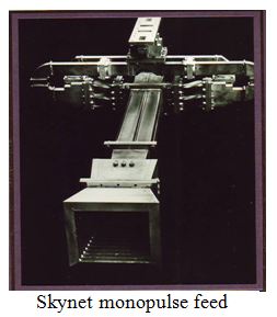The company ventured into Space Communications, participating in the design of the SKYNET satellite communication system. The antenna consisted of a parabola of revolution but using a very complex feed, needing to provide monopulse tracking of the satellite. The system operated using circular polarisation with one hand of CP transmitted from the terrestrial station with the opposite hand transmitted from the satellite station. The system worked in polarisation diversity. The feed was mounted behind the main reflector and directed toward a ‘sub’ reflector mounted at the focus of the parabolic reflector, thus producing a cassegrain antenna. Photographs of this appear in the SATCOMS section of this book. When used for radio astronomy or satellite communications, cassegrain antennas have significant advantages over conventional dishes, i.e. they have a feed at their focus, where the transmission line losses are reduced; also ‘spill-over’ (energy lost round the edges of the dish) illuminates ‘cold’ sky rather than ‘warm’ ground. The antenna ‘Noise Temperature’ is thereby minimised, which is an essential requirement when needing to detect very low levels of signal against a relatively high level of background thermal noise.

SHAPED REFLECTORS (DOUBLE CURVATURE)

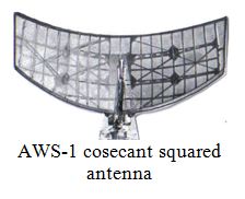In the late 1950’s, beams formed from parabolic sections could no longer meet ever more demanding operational requirements. The Decca AWS-1 naval radar brought to the market an antenna having a cosecant-squared elevation radiation pattern. The reflector’s horizontal shape was still basically parabolic, but the vertical section departed from parabolic, this departure becoming more pronounced over the lower sections of the reflector. The effect of this ‘distortion’ was to direct the rays from the feed horn to higher elevation angles thus increasing the radar coverage at these angles. The law that the beam had to follow was cosec-squared; this meaning that the power gain of the antenna (feed plus reflector) had to reduce according to the cosec2θ law where θ is the elevation angle with respect to the antenna. The advantage this brings is that the use of the available RF energy is optimised and the power is radiated into space only where, and at the level consistent with the system performance requirement. In operational terms a target flying at constant height ‘inbound’ or ‘outbound’ with respect to the antenna, will return a constant signal level to the antenna even though the slant range is changing. The antenna was linearly polarised. The AWS-1 antenna evolved into the AWS-2, which had the capability of a basic variable polarisation, linear through to circular. The purpose of providing circular polarisation (CP) was to reduce radar returns from rain and (possibly) sea clutter. It was from this antenna that the AR1 (land based surveillance radar) antenna was developed. The AR1 however, had a more complex system for deriving circular polarisation, this aspect being covered in section 15.4

Another example of a reflector having double curvature is the Decca harbour radar Type 32. This operated in ‘X’ band and had a large horizontal aperture of some 8m. The vertical aperture was in the order of one metre high and shaped to produce an ‘upside-down’ cosec2θ power gain pattern, the object being to detect small craft at large angles of depression. The first of these radars was installed at the harbour in Hamburg followed by an installation at Southampton. The radar utilised horizontal polarisation so it was possible to manufacture the reflecting surface from horizontal rods making the construction very simple. The rods were held in place by jig-drilled plates mounted vertically onto a riveted box structure.(See Chapter4.2)

PLANAR ARRAYS

Plessey Radar came late into to the planar array market, (although some work had started in their Microwave Group in late 1970), a time when most other major radar companies already had a planar array of some description on their books. The initial work on planar arrays had a very limited private venture (PV) budget. It was commissioned to study basic techniques and to design, build and test an array consisting of just nine elements.

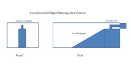
The element type chosen for this study was a waveguide of square section, suitable for transmitting CP, if a future need arose. It was at this time that the Research Centre at Plessey Caswell began producing microwave devices using silicon and gallium arsenide, so, in order to ‘push’ the technology, it was decided to design the planar array waveguide element to accept a solid state phase shifting device which, in principle, would lead to a ‘Phased Array’ rather than simply a planar array. The method used was to make the element in the form of a ‘ridged’ waveguide (see figure) where, ultimately, a solid-state device could be situated at the top of the ridge inside the guide. Although nobody knew at that stage how or what, a significant principle had been established. The project eventually ran out of money and work was discontinued, even before a suitable solid state device was available. However, this work came to the attention of staff at the Admiralty Research Establishment (ARE now known as DRA), at Portsdown, who were already studying phased array concepts for naval radars. This eventually led to collaboration on the MESAR project.

Plessey eventually broke into the planar array market with ‘COMMANDER’ and a number of its variants, using slotted waveguide elements grouped together to form a planar geometry.

For details of Commander see chapter 7.

COMES THE REVOLUTION.

MESAR (Multifunction Electronically Scanned Adaptive Radar)

It has been mentioned that Plessey came late to planar array technology and with no experience of phased arrays, but, when it did enter the phased array market it entered with a BANG!!!. Reflecting on the history of radar systems designed by Decca/Plessey, most of the systems evolved from predecessors, the Wind-finder radars to Weather radars, AWS1 through to AR1 and AR15 to AR5. The slotted waveguide feed of Type 80 spawned the slotted waveguide of the naval and marine radars, then onto AR3D and Commander and beyond. However, MESAR was a REVOLUTION.

The early dream of fitting a solid-state microwave phase shifter into a waveguide, as described earlier, was swamped by the MESAR concept where a complete, fully controllable microwave transmitter and receiver would be fitted into each radiating element. Under the control of software, the antenna would be capable of changing beam shape, from surveillance radar to tracking radar and even process all of these functions almost instantaneously. (During the MESAR years Plessey became Siemens/Plessey).

The MESAR programme was to bring forward all the important technologies and to de-risk future development, while proving the principles of the multi-function radar. These technologies were:-

• Improve efficiency and power output of Gallium Arsenide (GaAs) transmit/receive modules
• Decide optimum Active Array configuration
• Active Array heat management (module cooling)
• Develop software for Radar Control and Beam scheduling
• Develop Adaptive Nulling to counter multiple radar jammers (ECCM)
• Integrate all the new technologies into a functional trials system and evaluate the performance and demonstrate the principles of a multifunction radar (MFR) system.

The programme was jointly funded by PV and research grants from the Defence Research Agency (DRA) at Portsdown and was a collaborative programme. The DRA, as well as much of the MFR system studies and evaluations, carried out the weapon system work. The work on the Gallium Arsenide was carried out at Plessey Semiconductors at Caswell (Research) and Plessey Towcester (development and production of test transmit/receive modules), The Adaptive Nulling (ECCM) was carried out at Plessey Research at Roke Manor. Engineers at the Cowes site conducted the system design, configuration and performance analysis and the whole programme was managed and indeed, driven, from the Cowes site by a core MESAR project engineering team.

The MESAR 1 programme took place over a seven-year period resulting in trials at the DRA antenna range at Funtington in Hampshire, at which site all the main principles of the Multifunction Radar were proven. One aspect of the technology that was still in difficulty was the inability of the GaAs power stages to provide, at that time, the specified 2-watt output. MESAR went to trial using the GaAs driver stage as the output stage, which provided a module-power output of half a watt, sufficient only for trials on the antenna range. This shortcoming did not affect the multifunction or adaptive beam-forming (ECCM) trials. Meanwhile efforts to improve the GaAs output power stages continued at Caswell and Towcester. As MESAR 2 and SAMPSON will testify, this problem was overcome and indeed the requirement surpassed both in power output and efficiency.

The path to completion of MESAR 1 was not easy and many dark passages had to be worked through before emerging to the light. It must be said that even through the darkest of these the support from the MESAR team at the DRA (Portsdown) never wavered and this support was crucial to the eventual success of the project.

Following the trials at Funtington the system went to the MOD trials range at West Freugh, in Scotland. It was here that operating as a multifunction radar the system detected the release of a dummy missile (a cement filled bomb casing) from an aircraft and tracked the trajectory of both aircraft and missile. It became clear that, in radar, “things would never be the same again,”a new benchmark had been created. MESAR 1 was the foundation for all that followed, MESAR 2, SAMPSON and the rest, and that foundation it seems, is pretty solid.

15.4 CIRCULAR POLARISATION (CP)

The introduction of Circular Polarisation to Transmitted Radar Beams is based on the principle that circular polarised beams when illuminating spherical clutter, such as raindrops, would greatly reduce the possibility of reflections or echoes being returned to the radar Feed Horn and thereby reduce the possibility of displaying such clutter.

The RF input to the boom is split into two equal orthogonal vectors by the 45degree launching section. By varying the phase shift between the two vectors it is possible to provide linear polarization at 45degrees, through elliptical to circular polarisation.

The phase shifter, which has two dielectric vanes, is regulated from the operators control panel. The Boom Arm waveguide components have been designed such that two diverse frequencies feeding the antenna system have the same polarisation at any setting of the variable phase shifter, this by the inclusion of the Differential Phase Shift Equaliser (DPSE) section designed to compensate for any unwanted phase shift through any boom-arm components, (particularly the feed horn), which is introduced when the frequency of the transmission is changed.

The fin-loaded feed horn makes sure the beam-widths are equal for the orthogonal components of polarisation, which are vertical and horizontal, thereby ensuring that the amplitude distribution across the reflector is the same for both components thus producing equal beam widths from the reflector. The quality of the circular polarisation is preserved over the whole of the radar beam and when rain fills the radar beam this helps to improve the elimination of radar returns from the rain. Beam equalisation occurs because the finned horn presents a different sized aperture to the orthogonal components of the polarisation. The ratio of aperture size is the same as the ratio of beam-width factors for an aperture having first a cosine illumination (due to the vertical component of polarisation) and second, a uniform illumination (due to the horizontal component). The vertical component (red) fills the aperture as shown in light red. It cannot propagate into the top and bottom areas (white) because the waveguide is ‘cut off’ due to the fins. The same applies to the horizontal component (blue).

15.5. MOVING TARGET INDICATION (MTI)

EARLY DEVELOPMENT OF ANALOGUE MTI SYSTEMS AT DECCA RADAR

To remove ground clutter from the display of an Air Traffic Control radar screen the preferred signal processing system was a coherent moving target indicator (MTI).

Very stable transmitters and local oscillators were required for such a system, so that on reception the detection of the phase changes on moving targets and the non-phase change on static targets could be detected. The resulting measurements of phase change were compared over two (or more) pulse intervals so that static targets could be eliminated and moving targets be further processed for display to the operator.

A key element of the processing system was the delay line. In very early systems such as the MEW (Microwave Early Warning) -1940’s, a water bath was employed. Later systems like the Cossor ACR6 (1950’s) employed mercury delay lines.

By the 1960’s quartz delay lines were available (from the Corning Glass Company, based in the USA- and later from the Mullard Company in the UK).

Other adopted MTI features were frequency modulation and prf control by a servo system, giving more reliable triggering of the transmitter.

MTI system design work started within the Decca Company at Davis Road, Chessington, in 1960. Experimental work with hardware started when the Heavy Radar Laboratory moved to the Isle of Wight (1961) using the ‘LOTUS’ Transmitter and the LC150 Antenna.

A stable local oscillator was required (STALO) to allow the phase to be compared pulse-to-pulse. The first STALO was built at Cowes using a Mullard triode ‘Lighthouse’ Tube. Production systems went on to use American oscillator units with ceramic button triodes. The STALO needed careful anti-vibration mounts to avoid microphony and the tuning was mechanical. Video was suppressed during tuning to avoid cluttering the display.

The magnetron transmitter had a random phase pulse-to-pulse, so an IF version of the transmitted pulse was used to lock an IF oscillator (COHO) which formed a reference for the phase detector.

To keep the lock pulse free from TR cell ‘spike’ breakthrough the LC150 system had the transmitter fitted with balanced mixers, manufactured by the Mullard Company.

For many of the design team this was a first-time experience when using transistors in the circuitry. Unit specifications were written and the experimental units (for high frequency application) were made at the Decca Hersham site in Surrey and the displays and video units designed and manufactured at the Tolworth/Chessington Labs. The RF units and prf control designs, also the transmitter modifications, were carried out at the Company’s Cowes, Isle of Wight, establishment.

The first MTI production designs were aimed at the DASR-1 system where double cancellation was needed; so two carriers (narrow band FM) were put through one delay line.

The original objective was to loop the signals round without de-modulation, but spurious frequencies, which developed in the mixers, made this impossible. The standardised design was more acceptable with de-modulation after each stage of cancellation.

The prototype hardware (rationalised mechanical packaging of the electronic circuitry) was developed using a standard unit format. IF printed circuit units were built into two and three-inch screened boxes, with video and pulse forming hardware built onto open printed circuit boards. All were fitted into standard frames and cabinets for a professional finish.

The Decca display units at this time used germanium transistors and military specifications required temperature controlled cabinets. The designs developed on the Isle of Wight opted for silicon transistors, as high frequency versions were becoming available with good environmental specifications and a relatively low unit price.

The transmitter itself needed little modification as the hydrogen thyratron gave little jitter.

A problem to be addressed was that of ‘blind speed’ avoidance, as when the target Doppler is an exact multiple of the prf, the target would fade from the MTI. The solution was found in the varying of the inter-pulse period and re-aligning of the signals using an extra delay line.

The velocity responses of staggered prf systems were analysed by the mathematics team at Cowes, in some cases using computers at Southampton University.

The hardware in the MTI was not too complex, but the transmitter had to be modified by adding special charging diodes, to cope with the varying inter-pulse period.

The MTI system which was initially designed specifically for operation with the DASR-1, had to meet different considerations. The system design studies started at Davis Road at a time well before the general availability of computers. Estimated improvement factors were being calculated by counting millimeter squares on pencil graph paper. DASR-1 was a longer-range system with two antennas facing in opposite directions, each with its own transmitter triggered alternately at 250pps. This did not give enough pulses per beam width for effective cancellation. The answer was to fire the transmitters simultaneously at 500pps and store alternate traces in another delayed channel, thus allowing display at 250pps. The delay line had three channels; two were FM carriers for the MTI and a third (AM) for video storage. Each transmitter-receiver had its own MTI cabinet. Only one could be master for the prf control, so the two quartz delay lines were carefully matched to a fraction of a microsecond and were temperature controlled. The velocity response of the MTI was shaped, by using feedback. While this feedback technique had been suggested in an international paper, the actual bringing of a product to the market place was a world first by the Decca team. One additional de-modulator and video adjustment provided the specified impulse response.

However, the MTI system was finally fitted to what became the very successful AR-1 radar.

MTI test equipment was initially imported from America from where a 30MHz fixed and moving target generator was available. Similar equipment was later available from Sweden.

Jitter measurements were possible using a wire delay line to trigger a scope and there was also a STALO tester to check the oscillator FM. A cable delay line gave a delayed version of the IF Coho lock pulse as a useful on-line test signal.

These MTI systems gave the Decca Radar Company a strong foothold in the ground and naval radar field and paved the way for the application of digital MTI technology.

PPI presentations of the Isle of Wight and Southampton are shown, both before and after MTI processing with a synthetic (video map) coastline, overlay.

15.6. STRIPLINE

Strip-line is a form of transmission line consisting of a flat (strip) conductor of specific width and thickness suspended close to and parallel with an associated ground plane.

Electronic circuits consist of four fundamental components, resistors, capacitors, inductors and the means of interconnecting them. In the 1960/70s, at frequencies up to around 1GHz, these were usually discrete items assembled using carefully dimensioned wiring or printed circuit card. Microwave circuits working above this frequency, where the physical dimensions of the components and wiring start to become a significant fraction of a wavelength, most circuit elements were realised using either coaxial cable or waveguide. For high power applications, such as the connection between the radar’s transmitter and its aerial, waveguide is the only suitable medium since it is capable of carrying many hundreds of kilowatts of pulsed peak power. For low power applications waveguide is less convenient. It is bulky, heavy and does not readily lend itself to the construction of complex and intricate microwave circuits such as filters, modulators, switches, mixers and amplifiers, especially where there is a need to integrate many of these functions together in a compact assembly. Coaxial connection is suitable in some instances, but generally entails awkward and expensive mechanical constructions due to its having the ‘conductor’ completely enclosed within a cylindrical surround. Coaxial configuration carries energy in the form of a transverse electro-magnetic (TEM) wave. This TEM mode is one in which the electric field is symmetrically radial between the centre conductor and its surrounding metallic sheath. This is substantially so up to frequencies where the outer diameter approaches the signal wavelength, at which point other, more complex modes may propagate.

The mechanical restrictions of coaxial would be eased if, instead of being in a complete cylindrical surround the centre conductor could be supported in an open sided housing. Since the electric field in coaxial is always normal to the inner surface of the outer conductive ‘tube’ there is no harm done by cutting two diametrically opposite slots along its length. Imagine now that the two resulting semi-circular shells are flattened out. We then have the centre conductor suspended between two equidistant ‘plates’ usually referred to as ‘ground-planes’. Imagine further that the round centre conductor is also squashed flat and we have arrived at a basic form of STRIPLINE.

This stripline configuration, derived directly from a deformation of coaxial, is normally referred to as ‘Tri-plate’. Its preserved symmetry ensures that it still maintains TEM mode transmission and retains other properties characteristic of coaxial, such as a defined impedance and velocity factor. Impedance is determined by the ratio of strip width to ground plane spacing and the relative permittivity of the medium filling the space. Velocity factor is also a function of the permittivity. The benefit is that, unlike coaxial, the conductor (strip) geometry can be shaped in two dimensions. In other words the strip can vary in width along its length and branch sideways to form associations and contact with other strips and components. As with coaxial the centre conductor (strip) requires mechanical support to ensure it is held rigidly half way between the two outer plates. In many cases this is provided by a low-loss plastic material, (e.g. polythene) completely filling the space between the plates. Commonly the strip is of photo-etched foil attached to one surface of two equal thickness plastic layers, in the manner of conventional printed circuits. This technology, its supporting design rules and availability of suitable materials emerged in the late 1960s from a number of sources worldwide. The Microwave Group at the Cowes site in collaboration with Roke Manor established a predictable design and manufacturing process, initially used to make discrete items for experimental systems such as Tactical Transportable Radar 2 (TTR2). These prototype sub-systems were supplied to the Radar Research Establishment (RRE) at Malvern who were testing an active phased array; a very early forerunner of MESAR and SAMPSON.

A number of other components were designed using the tri-plate technique during the 1960s and 70s, most notably the AR5 receiver and the switching matrix for the DMLS antennas.

When Cowes adopted Travelling-Wave-Tube (TWT) transmitters to provide frequency-agility, air-spaced tri-plate strip-line was used to feed linear arrays.

TWT transmitters operate at peak power levels about a tenth of that from a magnetron transmitter. The correspondingly long pulses used to restore the mean power are coded so that high spatial resolution can be attained by pulse compression.

The microwave laboratory at Cowes, capitalising on the lower peak power from TWT transmitters, developed high power stripline for squintless antennas consisting of linear arrays of radiating elements (up to 80) fed in phase, with a tailored amplitude distribution across apertures of up to 5m.

This configuration was first used in the AWS6 (C-band) and Type 996/AWS 9 (S-band) Naval radar antennas and the Dagger (Ku-band) planar array. In these equipments the strip was used as a power divider (corporate feed) to provide the antenna’s horizontal aperture distribution. The strip was cut from brass or copper sheet under numerical control and suspended at intervals on small plastic pillars mid-way between aluminum ground planes, the separation being great enough to carry the transmitter power without electrical breakdown.

This was a neat way of providing a 2D radar antenna with an equi-phased power distribution and thereby avoiding the ‘squint-with-frequency’ associated with a series feed over the wide band of which TWTs are capable. A conventional horn and reflector antenna when used on a naval vessel required a massive masthead stabiliser.

This technology has been incorporated into other equipments but the introduction of the Active Phased Array, with their much reduced power level per element and internal phase control, has removed the need for large-scale high power stripline feeds.

Tri-plate is the most basic and manageable strip-line form. It is well shielded to prevent signal leakage and influence from external interference. Its TEM mode symmetry simplifies the design of transitions to other media (e.g. coaxial) and helps reduce unwanted internal coupling between otherwise isolated areas of the assembly. However, its usefulness for large-scale integration (LSI) of complex microwave sub-systems is limited by the need to contain all the circuit elements inside the two ground-planes. Clearly it would be more convenient if microwave LSI circuits could be laid out in a fashion similar to that of conventional electronic printed circuit assemblies despite the need to treat all the interconnections as transmission lines. To achieve this it is necessary to dispense with one ground-plane to expose the conductors and enable access to the electronic components that constitute the functional circuit. Doing this destroys the symmetry and without further adaptations would allow the resulting unconstrained stray field to radiate into the surroundings to the detriment of circuit function. By supporting the conducting strip on a thin sheet of material having a high relative permittivity (10 or more) the field is concentrated therein and leakage to the space above is minimised. A material commonly used for this substrate is high alumina ceramic or, in the case of microwave integrated circuits (MICs), a semiconductor such as silicon or gallium arsenide. This ‘one-sided’ version of strip-line is usually referred to as ‘microstrip’ to distinguish it from tri-plate.

Stripline technology based on microstrip has flourished with the introduction, over the last 20 years, of computer aided design and the availability of compatible components both active and passive. Development of the transmitter/receiver units for the SAMPSON radar depends completely on the latest strip-line techniques alongside custom designed semiconductor modules. Wherever microwave signals are processed STRIPLINE is the connecting medium of choice and has been used in one form or another in all our radar products since the 1980’s.

15.7. PULSE COMPRESSION

In the 1940’s and 1950’s the Magnetron proved to be an excellent low cost source of microwave power and ideally suited for radar applications. The device was developed during WW2 and made a major contribution to the UK endeavors. Interestingly, although having no connection with Decca, the device was developed by Dr Boot of Birmingham University, partly on the Isle of Wight, at the Chain Home Radar station located on St Boniface Down only a few miles from what was to become the Decca site at the Somerton airfield at Cowes.

However the usefulness of the Magnetron was limited, due to the nature of its operation involving resonant cavities to determine the microwave oscillation frequency. Its operation was similar to a church bell, when it was hit by the bell hammer (in this case by a large high voltage pulse), it would ring (oscillate) and could be heard miles away. The bell sounds the same pitch (frequency) each time it is rung, but if you listen very carefully with a sensitive ear you will hear tiny changes of pitch. The Magnetron is the same and there are very small unpredictable changes in the frequency of the pulse each time it transmits from the radar. This proved to be a serious limitation, especially for military applications of radar.

In the 1950’s there was a demand from radar users for improved performance. Civil air-traffic management wanted to remove the unwanted reflections from the ground and rain that tended to obscure the echoes from passenger aircraft on the radar screen.

Military users wanted to see the small fighter aircraft (which returned a much smaller echo than the large passenger aircraft) at much greater range. At the same time they needed to be able to see two or more fighters very close together as these tended to appear as a single blob on the screen. Attacking aircraft could exploit this weakness by flying one aircraft exactly below another so that there appeared to be only one aircraft approaching. Special optical systems were developed for use by the pilot in the higher flying aircraft to enable him to achieve the difficult feat of keeping station exactly above the lower aircraft. When the defending aircraft engaged the attackers the pilot would be surprised to find two aircraft and would be at a serious disadvantage. Another technique used by attacking aircraft was to drop millions of tiny pieces of aluminum foil to form a large cloud, which behaved like rain and its large echo obscured the small aircraft hidden in the cloud. This was known as chaff or window. Many other military techniques were developed to exploit the weaknesses in the then current radar performance.

Removal of the unwanted echoes from rain and chaff (or clutter as it was known) was tackled using Moving Target Indicator (MTI) equipment which measured the speed of the echo and rejected the slower moving rain and chaff returns. The effectiveness of MTI was however limited by the small random changes in microwave frequency and did not fully satisfy users who needed even more rejection of the unwanted returns. Radar engineers tackled this problem using innovative new technology and Decca engineers turned this into practical radar systems, firstly in the AR3D and later in the new generation of naval radars starting with AWS-5.

Two major advances were required. Firstly the Magnetron was replaced by a ‘Driven Amplifier’ Transmitter, which eliminated the unwanted variation in oscillator frequency of the Magnetron and enabled better clutter cancellation. Secondly, ‘Pulse Compression’ was introduced to achieve much more accurate measurement of range, especially as the driven transmitter had to operate with a much longer pulse, which would have resulted in unacceptable range accuracy and resolution of closely spaced aircraft or missile targets.

Driven transmitters as the name implies, were used to amplify low power and provide a very precise frequency source to generate a stable transmitter pulse. This produced exactly the same frequency from one pulse to the next. The Driven transmitter was used with MTI to achieve a much greater cancellation of unwanted clutter signals than was possible with the Magnetron. The limit of cancellation performance was determined by the small amount of noise, which contaminated the Driven Transmitter pulse. There were two main types of Driven Transmitter device – the Klystron (one was specially developed for AR3D by the Thorn-EMI laboratories at Hayes, Middlesex working with Varian in San Francisco and the scientists at Stamford University) and the TWT (which was used in the AWS-5). However, whilst these new transmitter systems allowed excellent clutter cancellation, there were serious drawbacks for the radar system engineers.

Driven Transmitters were capable of producing very high powers. This satisfied the military need to see much smaller aircraft, but did so by transmitting a much longer pulse (typically 100 times the duration of a Magnetron pulse) leading to unacceptable overlapping of the returns from targets closely spaced in range. The technique of pulse compression was developed to overcome this problem which led to Driven systems that had range resolutions some 10 times better than those obtained with the Magnetron.

Essentially Pulse Compression involved coding the transmitted pulse with a varying frequency with time (swept frequency pulse) and then using a radar receiver, which optimised the code and converted the long pulse into a very short pulse, less than one-hundredth of the length in time of the transmitted pulse. This was achieved without loss of energy, so that the narrow pulse grew in height as it was reduced in length, thereby enhancing the ‘signal to noise’ ratio and enabling small targets to be seen against a background of noise and clutter residue.

For those interested in mathematics this process was a fascinating application of Fourier transforms and convolution theory that led to much mathematical work optimising the system. Much of this was done using pencil and paper and analytic techniques supported by numerical work with the help of a computer. At that time there were no computers available at Cowes and much work was undertaken by Decca mathematicians using the computer facilities at Southampton University.

The transmitter driver used conventional, highly accurate, swept frequency technology to generate the pulse, which existed from the development of FM radio transmitters. The difficulty was the receiver device, which had to be specially developed.

Simplistically, the receiver device can be considered as a filter, which delayed the incoming swept frequency by varying amounts (longest delay of the frequency at the start and shortest for the frequency at the end) so that all the frequencies arrived at the output at the same time and produced the short output pulse. The short pulse length is about equal to the inverse of the amount of frequency change in the received swept frequency pulse. As an example, idealistically a change of 10MHz in the swept frequency pulse (of typically 10Sec duration) would produce a compressed pulse of 0.1Sec duration, enabling targets spaced only 15m apart in range to be resolved.

Initial work on pulse compression centered on the design of devices for the receiver system to compress the incoming swept frequency pulse. The first systems used “Bridged-T” filters, which have a characteristic variable delay with frequency. Sets of these filters, tuned to different frequencies, were cascaded to achieve the desired overall frequency characteristic required to ‘match’ the transmitter waveform. These comprised inductors (coils of copper wire wound on ceramic tubes) and high quality capacitors (silver plated mica insulation) all of which had to be very accurately made, in order to have precise impedance values and resonant frequencies. These were difficult to set up to be an exact match to the transmitter waveform, but were nonetheless made and used for the early experimental versions of pulse compression radar.

The break-through came with the discovery that acoustic waves could be generated from the received electrical signal (using the piezoelectric effect) on one side of certain crystals (such as quartz and lithium niobate) and received on the other side using special frequency selective sensors, to create the desired variable delay (dispersive) characteristic and output the compressed electrical pulse. This is analogous to a prism used to create a rainbow from white light and vice versa – hence the adoption of the optical term ‘dispersion’ to describe the function of these devices. Early devices used ‘Bulk Waves’ which were transmitted through the crystal. These were later replaced by ‘Surface Acoustic Waves’ devices (SAW), which travelled across the surface of crystals (cut at a special angle). This work was carried out at the Plessey Research Laboratories at Caswell. These laboratories also produced the devices used in the early versions of the AR3D.

Much work was done to refine the design of the surface wave compressors and excellent radar performance was achieved. However these were, much later, replaced by today’s high-speed digital filters.

15.8. THE INTRODUCTION OF DIGITAL AND SOFTWARE PROCESSING INTO RADAR SYSTEM DESIGNS

INTRODUCTION

The ‘invention’ of digital and software engineering, their application and development in Radar Systems is covered by several topics, this being spread over some five decades. It has therefore not been possible to stay within a strict chronological order when the considerations, in time, cut across each other.

The main topics covered are:

The Early Days - The formation of the original Digital/Software Groups and their initial developments.

Projects of the early days - A description of the first project application on the HF 200, together with a mention of early Analogue to Digital (A/D) converters and their power supplies.

Component Development - A brief history of the key digital components with an indication of their impact.

Software Systems - A brief history of the key software processors and applications.

Key Functions - An introduction to some of the hardware and software taken on, or invented in the Digital and Software System Groups within the Company.

Annexes - Major functions warranting further explanation are recorded in 6 Annexes to this section.

THE EARLY DAYS

The development of ‘software’ took place separately to meet the requirements of ‘Display Systems’ and ‘Radar Systems’. The Display System Development was centered at Hersham/Tolworth/Addlestone and finally Chessington, in Surrey, whilst the Radar System activity was mostly confined to the Cowes site on the Isle of Wight.

HERSHAM/TOLWORTH/ADDESTONE/CHESSINGTON– Computer Software Developments

In 1955 the Decca Radar Company had funds sufficient to diversify into the building of a commercial computer, this under the direction of the Decca Radar Research Director, at Tolworth. A design and manufacturing team was set up, initially at Malden Way before moving to Hersham and then Tolworth and Addlestone. A sales team was also set up at the Decca Head Office on the Albert Embankment, London.

The plan was to build a serial computer using shift registers constructed from ferrite cores and copper oxide diodes. Valve-generated pulses, at some 500kb per second, drove the cores. The technology failed through the poor forward/reverse impedance ratio of the diodes under pulsed conditions. The technology might have worked if semi-conductor diodes had been used but these were only just becoming available and too expensive at the time. While the project was still alive, papers were presented at an IEE Symposium on Computing Technology, including a paper on the Decca Radar core logic based computer. Other papers were presented on the use of cores in memories. At the end of the presentation one listener commented:

“Cores for stores, lets have more. Cores for logic better dodge it.” How right he was!

Permission was obtained to make use of the digital tape unit ‘know how’ developed on EDSAC l (Electronic Design Storage and Automatic Calculator) at the mathematical laboratory of Cambridge University. This allowed Decca to develop, build and market ‘twin tape units’ for other computer manufactures. Customers included LEO, Ferranti, English Electric and others. One of the others was the Cambridge University Mathematical Laboratory.

Another project for the team was for the Decca Navigator Company. The Decca Navigator system gave the position of an aircraft to great accuracy within a system of hyperbolic co-ordinates, but this information was only displayed in the aircraft cockpit itself. The Navigator Company awarded the Commercial Computer Development Team a contract to build an air-to-ground data link using tone modulated digital signals so that the display in the cockpit could be replicated on the ground. This system was capable of working in noisy signal conditions and dealt effectively with multi-path propagation problems.

The output from the Decca Navigator system, however, would have been more useful if the information was made available in Cartesian map co-ordinates rather than hyperbolic. This problem was solved, in mathematical terms, at the Decca Head Office. The Navigator Company developed ‘Omnitrac’, a small digital computer to do the job. Later ‘Omnitrac’ and the data link operated together.

Around 1956 Philco, in Philadelphia, produced the first surface barrier transistor. A technical visit was made by the Surrey based Decca computer team to see it. A few prototype transistors were brought back for experimentation and if possible the building of a bi-stable circuit, this was achieved. Shortly after this the Mullard Company came out with their first junction transistor, the OC70 and Decca bought some of them.

A paper in the radar field suggested that a plot extractor could be realised using core matrix store technology with a special purpose signal processor. While such an approach was attractive and feasible, it was thought it would be much better to use a standard computer and carry out the plot extraction using software. At the time computers were not fast enough to do this, but clearly they were going to get faster. Nonetheless, it was thought computer technology, especially core matrix stores coupled with registers would be the way to go. The Company provided funds (£10,000) for the construction of a four bit fixed programme computer with a small core store for testing core store/transistor technology. The team named the equipment ‘MAUREN’ (May Add Up Really Easy Numbers). The project was successful and was demonstrated to visitors as a means of attracting further funding.

As more sources of data were applied to computers, core matrix stores were employed as buffer stores to enable the various data rates of peripherals to be readily accommodated by the computer. Decca Radar Research Laboratories already had close links with GCHQ and the Airborne Radar Team at Hersham had produced a miniature radar signal tape recorder for them; GCHQ also had a requirement for a buffer store and placed a contract to build two more of them. This was the team’s first contract for the new technology on a commercial basis. The group now had a commitment demanding continued funding. The buffer store was successfully created and delivered as the Decca Type 727 processor.

Decca Off-line Data Processing Equipment

There was a requirement in Digital Processing Systems for off-line processors which translated information from one medium to another e.g. punched paper to magnetic tape or matched the data flow from one type of equipment to another, complete with procedures for error detection or correction.

Equipments which would have been embraced were:-
Magnetic Tape – Punched Paper Tape – Punch card
Radio or Line Digital Data Links – Printers -
Keyboards – Digital Computers

DECCA TYPE 727 PROCESSOR – Designed for handling data between magnetic tape units and data channels at 100,000 characters per second.

Today this amount of storage can easily be provided on one silicon chip. Hopefully there will be the same degree of advancement in computing over the next 50 years.

Parameters

Input data rates	0 to 1 Mc/s.
Output data rates	0 to 1 Mc/s.
Ferrite variable storage capacity	1,024 or 4096 word modules. 1 to 24 bits per word
Access time	2.5 2.5 µsec. Minimum
Cycle time	6 µsec. Minimum
Programme storage	512 word plug in modules
Access time	2 µsec. Minimum
Cycle time	4 µsec. Minimum

REQUIREMENT SPECIFICATION

To operate between a fast start/stop magnetic tape unit and a computer as a buffer store. Information able to flow in either direction at any one time.

• Computer data rate (in and out) 1000,000 characters per second
• Tape deck data rate (in and out) 30,000 characters per second
• Input channels 6 or 7
• Output channels 6 or 7
• Block Length Variable, 50-1,024 characters
• Storage
  • 2 Variable stores – each 1,024 characters
  • 7 Bits per character – Access time 4µsec.
  • Cycle Time 9µsec.
• Special facilities
  • Echo check when writing on tape.
  • Parity generation and checking.
  • Block length check when reading from tape.
  • Reading backwards from tape.

Thoughts turn to how this technology could really be used in radar systems. If the computer had a core store it should not be necessary to have another core store as a buffer. This question was considered and the result was the ‘Direct Integration of Digital Computers’. This arrangement meant that instructions were provided both for the programmers and for the peripheral equipment and each were treated in a similar way in ‘microprogrammes’. It greatly increased the speed at which inputs and outputs to and from peripherals could be handled. The microprogramme was an efficient and structured way to execute arithmetic and logic operations within the computer.

There was at this time some rivalry within the Company between the Display Group at Tolworth and the Hersham based computer group. It was notable the way the Hersham group drew a diagram of a radar display system with the computer always placed in the middle of the picture, whereas for the Tolworth produced drawings the radar was always in the middle with the computer as a peripheral device!!

Around 1960, RRE awarded Decca Radar a contract to build a computer centred pilot air defence system. The project was given the code name ‘MERVYN’ but was known in the computer group as the Digital Data Processor (DDP). The design was based on the technology used when supplying the buffer store to GCHQ.

Architecture:	24bits parallel
Clock Speed:	1MHz
Switching Elements:	Germanium Transistors
Memory:	2048 Words of 24bits Ferrite Core
Control:	Germanium Diodes Micro Programmes

Germanium diodes and transistors were becoming available at reasonable cost. While the clock speed of 1MHz sounds very low by today’s standards, the operating programmes were written in machine code, so did not slow down the hardware as high-level languages do today. As is well known: “Intel giveth and Microsoft taketh away”.

The manufacture and construction of the machine proved more difficult than the designers of the hardware expected. The Managing Director instructed a senior manager, who had considerable experience in large systems, to investigate the situation. He discovered that there were no unit test specifications, no unit-testing going on and no test Inspectors. The designers were put to work to produce test specifications, test rigs were then constructed and Test Inspectors were drafted onto the team.

The software for Mervyn was written by CERI under a sub-contract operation, an unusual procedure at the time in programming, and required the development of special quality assurance procedures; these were again produced in software. ‘Mervyn’ was moved from Hersham to Tolworth and was set-up together with operator consoles as a fighter control air defence system. The installation was enhanced by the addition of an Ampex videotape machine which played back recordings of radar signals allowing realistic demonstrations of fighter interceptions. The Tolworth system was demonstrated to many potential customers and led directly to a number of contracts, many of high value. Some of them are briefly described in this chapter.

‘MERVYN’ (The DDP or Digital Data Processor) may have been the first computer to be built in the U.K. using semi-conductor technology. EDSAC 2 was of similar architecture but used registers of miniature valves. At this time the number of teams working on computers in England was very small and everyone knew what everyone else was doing, except for security aspects. The only place at the time where there was interest in transistors for computing circuits was the Harwell Atomic Energy Establishment, but as far as is known no such computer was completed there.

A turning point for Decca Radar in the computer application business came when the Company lost out to Marconi who were contracted to supply a display system for Sweden. MERVYN became the trump card for Decca to play for the next system and the computer design team were asked to visit Sweden with their thoughts on the use of data processing in air defence. However, no contract was immediately obtained from Sweden. Without the MERVYN model and its influence on RRE it is unlikely that Decca or Plessey would have received many of the contracts that were subsequently placed with the Company.

In 1963 Decca Radar secured a contract, to supply 6 small data processing and display systems to work with Sperry ANTPS-34 transportable V-beam radars, which the RAF had ordered. The system was based on the Decca Navigator Omnitrac computer. All the software was written ‘in house’ by a one-woman programming team – the ideal size! The programme had to be fitted on a drum store with just 1024 24-bit words of space. 1023 were used. A complication was that the circuits in Omnitrac, which selected the tracks of the drum, (probably 8 of them) were used to select the input/output ports. This meant that the programme instructions had to be placed onto the right track for the port being used at the time. The system had four operators, each equipped with a plan position indicator (PPI) and a rolling ball, which allowed a cursor to be positioned over the two blips of a target. Each blip position was entered into Omnitrac. The programme calculated the height of the aircraft from these inputs including allowance for the refraction of the radar’s beam in the atmosphere. The result was then provided as an input to a digital display along side the PPI.

Around 1963 the U.K. Government restructured their armed forces in the light of the cold war and their contractors were restructured correspondingly. Decca Radar was contracted to supply the displays and Ferranti the computers. The contract ‘NIGEL’, being a follow-up to MERVYN was cancelled and Decca’s Displays and Computer Groups were merged. Despite the setback resulting from the U.K. Governments decision, most key members of the Hersham Computer Group joined Plessey Radar, as the ‘Non-Marine’ part of Decca Radar had become. In many cases Air Defence Contracts of the time set Plessey Radar having overall systems responsibility.

GL161 - for the RAF used Elliot computers with Plessey software and display consoles.

‘Hubcap’ - for the Royal Australian Air Force used Marconi computers, CEIR/Logica software, Westinghouse (A1) TPS-27 3D Radars, Whittaker secondary radar, Selenia microwave links and Plessey display consoles. The system was designed to be transportable in a C130 Hercules.

Royal Navy – Command and Control Systems for Frigates, of Plessey Radar design, used Ferranti computers with ASWE having overall system responsibility.

COWES, ISLE OF WIGHT ACTIVITIES relating to computer/software developments

Further important moves in the computer/software field took place on the Isle of Wight. The Company having taken control of the old airfield site at Somerton in the April of 1959, then set up a new department, to undertake advanced studies with the aim of enhancing the Company’s products. It would be a forward thinking department wedded to new ideas related to the rapidly advancing technology, this included both hardware and in due time, software.

The next few paragraphs do not relate directly to the development of computers and their software but tell of how the hardware was constructed on which programmes would be run.

In 1960 work was under way, initially with a limited approach to semi-conductor design and their applications. Practical design of products assimilating these new ideas would first require an understanding of the fabrication and production of semiconductors i.e. transistors, etc. Companies such as Texas Instruments would dope surfaces on Germanium slices to produce individual transistor chips, carefully scribing and separating them, mounting them on headers and attaching (welding) them to header external leads with gold wires. This assembly was then covered in a waterproof paste and encapsulated in a metal can. Hence the three-legged transistor that is still in use today.

It was thought that after all this careful production, even allowing for reliability (yield) of these units, the recipient would use them in digital designs by combining them on printed circuit boards. It was glaringly obvious that if the combining could take place at the ‘slice’ level then an unnecessary step in low yield, large size, slow transmission speed and eventual shorter life would be avoided. At various visits made by the Cowes based team to the producers of semi-conductors, the idea was usually accepted and in one case eyebrows were raised; this was a short time before the commercial introduction of the fist integrated RTL (Resistor Transistor Logic) units.

Before the eventual commercial adoption of the integrated circuit by various manufacturers design work was undertaken in-house at Cowes to test the possibility of producing multi-connected transistors (bi-stables, switches and impedance converters) on a single slice of Germanium or silicon. All the equipment plus materials (Germanium, silicon slices and chemical processes) were obtained and after a few weeks slices were fabricated in the form of diode arrays.

In parallel, experiments in semiconductor reliability were undertaken where, against all advice, transistors (principally of OC 71 fame) were beheaded by removing their glass cover, washing the header in acetone and remounting and encapsulating them in a perspex block. (A forerunner of the Integrated Circuit) These were electrically connected, switched under temperature controlled conditions and continually recorded. In various forms, this went on from 1960–1965. No failures occurred but the experiments were discontinued, only for space availability reasons. However the concept of integrated arrays had been born.

In 1960 construction began on a prototype fixed purpose computer, known as FRED Mk.1. It was to herald the future design of radar data handling using transistors and only 2 values of resistor (330  and 1K2 ). Germanium (pnp) devices, because of their low switching threshold (typically 200mV), were used for FRED Mk.1 but FRED Mk.2 (14 bit) used Silicon (npn) devices and a higher voltage ( 650mV).

Using their characteristic Peltier/Seebeck, effect commercial refrigeration elements were used to provide smooth low impedance power supplies for FRED Mk.1. By heating one surface of the element and cooling the other with water, a potential difference was obtained. This realised voltages of approximately 300mV per element and by combining these it was possible to produce the required supply voltages of 300mV and 1-2 volts. Not only was this successful in producing smooth (noiseless) DC supplies but the device size (approx. 300mm x 60mm x 60mm) had an effective massive capacity of some 3 Farads. This was ably demonstrated to the engineering team based at Tolworth (who did not believe in the concept of FRED) although after switching off the power to the element heaters, it was seen that the machine continued to run for over 3.5 minutes! Although this generator was not taken up it did realise the success of FRED and its eventual furtherance of fixed computers in later Decca/Plessey radar system designs.

FRED Mk.1, as stated, was composed of Germanium Transistors operating in bistable/switching/impedance converting mode. Speed was a limitation and hence silicon was finally chosen for FRED Mk 2, where clock speeds of greater than 5 MHz were obtained. Machine code firmware was used to digitise the height information (derived by the HF200 radar) and produced an output of binary/decimal information. This was later incorporated into unit designs.

In 1964 Automation was also investigated. A fixed purpose computer was commissioned and built to reduce the manual (time consuming) aspect of waveguide production. This was well ahead of its time and although the method was not adopted (short term) it further acquainted designers with the concept of computer control.

When Decca was taken over by Plessey to become Plessey Radar in 1965, the department became APG (Advanced Product Group), again headed by Bob Matthews and under the General Engineering Manager Ron Burr. The greater resources of Plessey then enabled APG to expand and further their research and development of new products and digital techniques.

About this time LASERS were beginning to make their mark, both gas and semiconductor. A sub-group was set up to investigate and promulgate ideas for their use. A brief summary of the Point Visibility Meter (PVM) and the Ceilometer appear under the Environmental Sensors Chapter 14.6. although the design of the Slant Visual Range Monitor (SVR) is dealt with here.

SLANT VISUAL RANGE MONITOR (SVR)

RAE Farnborough contracted PRL to develop a laser based system to measure the visibility up a glide-slope. The system had two transmitters, an infrared solid state laser producing a 20Sec infrared pulse and a NdYAG high power laser producing a 5 mW infra-red pulse which was frequency doubled to produce a 0.5 mW 20 nano-sec pulse of green light. This was used with a narrow band optical receiver filter to detect the Raman atmospheric backscatter. The receiver used a silicon diode for daytime use and a photo multiplier for nighttime.

The solid state laser was used to measure the normal backscatter from the mist or fog.

For comparison and calibration a transmissometer with optical corner reflectors was located alongside and vertically up a 100ft tower. The selected receiver was mounted at the focus of a 2 ft diameter parabolic mirror and the solid- state diode transmitter at the focus of a 1 ft diameter spherical mirror, the high power laser fed out directly. The mirrors were mounted on a WF3 chassis to allow it to point in any direction including vertically.

The system was developed at Cowes and then operated by Plessey staff at Farnborough for a year, they often having to work at night, this when fog usually occurred.

PROJECTS OF THE EARLY DAYS

THE HF200 ALLOCATOR – The antenna of the HF200 Height Finder radar radiated patterns with a narrow vertical and broad horizontal beamwidth. The aerial nodding up and down at some 10 cycles per minute could also be rapidly slewed in azimuth to face the bearing of a target whose height had to be ascertained. The Height Range Indicator (HRI) Display would show Height against Range on a CRT. The required target was marked on the height operators’ display by a strobe that was initiated from a Plan Position Indicator (PPI) operator's console. Initiating this strobe caused the height finding radar to swing around to face the target azimuth (Azication). The height operator aligned his cursor to the centre of the indicated radar paint on his height display and the height was then calculated and displayed on an indicator adjacent to the operator console that had requested the height. Typically at RAF Boulmer two HF200s serviced the PPI height requests.

An equipment designed by the Advanced Products Group (updating a product that had employed Post Office Type3000 relays) came to be known as the Sub-Allocator. It carried out the control function of accepting PPI height requests and routing them to the next available HF200 antenna. The sub-allocator accepted the height voltage from the HRI operator and calculated the actual height based on the target angle and range. Previously the height data was displayed as an open resource, the new arrangements routed the data, via a data highway to a display local to the PPI requesting the data. The sub-allocator was a fixed programme controller which included designs that had been developed from the basic idea of using a 330 ohm resistor and general purpose switching transistor 2N706 or similar. The power rails were 3.3V for the basic circuits. All the required logic of AND, NOR, Bi-stables and timing circuits used the same two component types. Control interfaces with other radar equipments were achieved using small low power relays. Each PPI was fitted with a height display unit connected to the Sub-Allocator via a digital highway. These units accepted height requests at the PPI consoles. The Sub-Allocator queued the requests and when an HF200 antenna became available, made the control connection with the Main Allocator for the HF200. The Display units each had indicators to display basic and relative height information when involving two targets. Main Allocator units were also designed using the same ‘two component’ logic as the Sub-Allocator. The Sub-Allocators went on to provide continuous service until replaced by the Company’s 3D Radars. The ‘two component’ circuitry was never intended to be of ‘high speed logic’ but was very easy to implement and provided a good reliable means for the particular project. At this time the TTL family of 7400 series logic was becoming available but too late for the Sub-Allocator.

ANALOGUE TO DIGITAL AND DIGITAL TO ANALOGUE CONVERTERS

In the Advanced Systems Group these converters were known as ANDIs and DIANs, it being easier to say than the full title! The requirement for these units featured not only in the sub-allocator for HF200 but also in a number of other projects, one such being the provision of a remote display with video and turning data, via radio link, for Hong Kong Airport. The remoting was based on synchro and servo devices and the ANDI provided the conversion of the synchro output voltage to digital form for transmission as a serial bit stream. At the remote end the serial data was de-serialized and converted to an analogue signal for use by the display servo. The conversion rate was in the order of Khz and the ANDI used a successive approximation method for conversion. The modern version of this is available as an integrated circuit, but then it was implemented by a number of discrete circuits. (Details of operation of this type of Analogue to Digital Converter are readily available on the Internet.)

THE MOVE TO DIGITAL TECHNOLOGY IN RADAR SYSTEMS

The use of commercially available Integrated Circuit logic in the processing of real-time radar signals began at Cowes with the Digital Moving Target Indicator (DMTI). There are aspects of the use of integrated circuits that only became apparent when the design team started work on this project. From an engineering point of view the immediate effect of using a large number of logic gates together had a dramatic demand on power supplies and power distribution within the card frames. The power consumption presented by the circuitry required a very high current at a potential of only 5 volts, this giving rise to a large voltage drop in the power unit supply lines.

The use of a motherboard that housed the circuit cards, including an earth plane, became the norm. Shielding of signal lines was necessary to control mutual interference. The timing of a frame of logic cards required a new set of Timing and Control cards, these became ‘standards’ and could easily be adjusted as required to provide a flexible design arrangement.

The analogue to digital converters, needed to digitise the video going to the canceller, were high speed ‘Sample & Hold’ units purchased from the Analogue Devices Company, it having been decided that it was not viable to develop ‘in house’ converters in the project time scale.

THE DIGITAL GROWTH YEARS

Component Development - As always with new technologies it is in the early years that the possibilities are seen and therefore shape the future. This is true for both the device manufacturers and the device users. In the field of digital components one of the first major decisions was whether to use germanium or silicon as the basic material on which to create devices. Silicon was selected, predominantly because of its real advantage in speed and germanium was almost dropped completely. This proved to be a sound decision as Silicon went on to provide the majority of the core devices right through to the current day, this in spite of several periods when it was suggested its life expectancy was limited. New techniques continued to be invented, allowing both device capability and device speed to maintain improvements in line with market demands. It is worth mentioning that at one point it was felt that silicon would peak at a speed of around 25 to 30 MHz. Currently there are silicon-based components on the market with internal clock speeds in excess of 1 GHz.

One of the alternatives, Gallium Arsenide, has had a number of attempts at taking over from silicon. Although it has always offered dramatically improved speed operating into the GHz clock speeds, it has always remained expensive and therefore its use has remained in the more specialist ventures, but not for general digital engineering.

Early circuits were designed using discreet transistors, but moved relatively quickly into ‘integrated circuits’, which were still transistor based but offered a variety of functions within the devices. There were three steps made in fairly quick succession in integrated circuit design. These were RTL (resistor transistor logic), DTL (diode transistor logic) and finally TTL (transistor transistor logic). TTL was seen to offer the most potential for growth and be the most cost effective. It quickly became the industry standard for logic circuits, with the range of devices continuing to expand over a number of years. Other alternatives appeared over the years, most notably CMOS, which was used within Plessey Radar on the Microwave Landing System (MLS) development. However TTL remained in use from the very early seventies through to the late 1980’s.

TTL was supported by a number of specialist components. The most important of these were ‘memory devices’, as these allowed a complete new range of processing elements to be realised. They were originally developed in two types, dynamic storage (RAM) and programmable (PROM). The RAM was used as working memory for activities such as the temporary storage of data in functions such as MTI or Pulse Compression, and the PROM’s were used for timing sequences and data conversion. Two other key components were the Analogue to Digital (A/D), and Digital to Analogue (D/A) converters, which were fundamental to the growth of digital signal processing circuits.

The speed and functionality of the TTL component range and the storage components continued to be expanded. By the end of the 1970’s the complexity of components had taken a further quantum step with the creation of a number of new digital component sets. These were the Programmable Gate Arrays (PGAs). The original devices were ‘manufacturer programmable’ only. These were used with great success in the DAGGER system where just a few complex customised devices provided the majority of the control, timing and signal processing for the radar.

Over time a family of Gate Arrays were produced that could be dynamically programmed by loading firmware into the device (Field Programmable Gate Arrays FPGA). This range of devices has continued to expand through the late eighties and nineties. They are now the basis of virtually all of the radar digital design, with devices equivalent to many millions of gates operating at speeds of several hundreds of MHz.

Due to the enormous capacity of each device the number of connection pins has had to increase. The majority of TTL devices were ‘14 pin’ with the largest devices being ‘24 pin’. Current PGA’s can have in excess of 500 connections, although they are no longer pins that are fitted through holes in printed circuit boards, but are connecting pads or ‘balls’ that are surface mounted to the board.

It has to be mentioned that in parallel with the circuit design activities there was considerable activity in the creation of the printed circuit boards themselves. This was originally carried out by laying black tape on melamine and then photographing it. As component densities and pin counts increased and track widths decreased this became impractical. By the late 1970’s this process had been automated onto ‘workstations’ running commercial software for component placement and track generation for the circuit boards.

In parallel with the growth of digital components, software processors were also being developed. It was not until some time in the mid 1980’s that they became fast enough to take on the real time signal processing functions. Prior to that ‘track extraction’ and display systems tended to be the only areas carried out in software. By the year 2008 standard commercial processors were fast enough to take on virtually all of the radar processing requirements. The following section tracks the development of the key software processors and systems.

DEVELOPMENT OF SOFTWARE PROCESSORS AND SYSTEMS

Software Systems - As mentioned above, over a thirty-year period there was a gradual migration of functions, implemented in dedicated digital hardware, into software systems. In the early days of using software it was confidently expected that within a short time, as host processors increased in power, software would take over all the major functionality. The reality was that it was much more difficult than was anticipated and even today there are areas which are still to be conquered.

The implementation of software was driven by the availability of host processors and a brief chronology of how they have appeared in the company’s products is appropriate. During the late 1960’s mini-computers (as opposed to main frames which had been around for a decade or so) began to appear on the market, two of the most notable being Data General’s Nova series and the Digital Equipment Corporation’s (DEC) PDP products. It was quickly recognised in Plessey Radar that these devices could be used advantageously within radars and indeed in one case (automatic tracking) made it possible for the first time to incorporate the function within a commercial radar. AR3D being the first product, made by Plessey Radar, which included a mini-computer and this was used for some of the control, calibration and all of the tracking functions.

The 1970’s saw the ‘Microprocessor’ appear on the market and a Plessey company (Plessey Microsystems) began to develop and market its own microprocessor – ‘The Plessey Miproc’. Microprocessors were used, amongst other later applications, for the control of the transmitter in the AWS-5 Naval radar.

During the early 1980’s it was perceived that the commercial processors on the market were going to take a long time evolving before they would be capable of hosting the very intensive signal processing functions in a radar and it was felt that a considerable commercial advantage would come to the radar company that had access to such a device. In response to this situation a programme of work, JP3 (Joint Plessey Parallel Processor) was started in 1986 to fill this gap. Initially this was based on using a large number of the new ‘Transputer’ devices, but later incorporated the I860 processing chip to handle the bulk of the calculations leaving the Transputers to undertake the control of the board and the organisation of the data. It is interesting to note that Marconi Radar had come to the same conclusion and were simultaneously developing their own processor board for signal processing (they stayed with the Transputer). In the early 1990’s the parallel processor boards were incorporated within a product (a long range air traffic control radar – ROUTEMAN - for NATS).

Simultaneous with the above development was the arrival of single board computers based on ever more capable processor chips that were being developed by Intel, Motorola, INMOS and others. These were adapted by Plessey Radar to host functions such as plot extraction (the PLESSEX plot extractor being a good example) but were not yet powerful enough to take on the processor intensive tasks of background averaging and Digital Pulse Compression. It was with the arrival of the very high performance processor boards in the 1990’s, such as the one from Mercury Computers, that enabled these (almost final) frontiers to be undertaken by software.

The advantages that come from the use of software in the radar environment are, great flexibility, easy changes to the functionality, independence from the hardware platform and quick development. However this proved to be much harder to realise in practice. It quickly became apparent that to achieve these gains and in particular to be able to make the software reliable and testable, working practices had to change and change fundamentally. Thus the early days of an engineer penning a few dozen lines of assembly code one afternoon had to be replaced by the development of a major department using industry standard high level languages and writing structured software in accordance with the emerging software development methodologies.

KEY FUNCTIONS

Throughout the life cycle of digital and software development in radar there have been a number of key steps, which allowed important processing functions to be realised. Some of these functions are sufficiently important to warrant an explanation of their own and a simple block diagram of a radar system is shown, to help illustrate.

The functions that were suitable for digital or software designs are shown highlighted with Signal Processing expanded to show some of its key functions. Signal Processing, Plot Extraction, and some aspects of Control and Timing all operated at radar range cell rate. As a result, initially they could only be implemented in discrete digital designs, whereas Track Extraction and Display sub-systems operated at slower data rates and were implemented directly into software.

A number of theses functions are sufficiently complex and important to warrant an additional commentary, which has been included as Annexes at the end of this section. Going through each of them in turn:

CONTROL and TIMING was the first main function to be given over to digital designs. They involved a certain amount of high-speed activity and were initially implemented predominantly using counters and gating circuits. A good example of this is the HF200 Allocator system described earlier in this chapter.

A to D CONVERSION was essential in order to carry out any processing of analogue signals in digital circuits. In the early days, when only limited functions could be carried out in digits, signals were often converted back to analogue part way through the processing. In time commercial devices became available with the resolution and speed required, but it was not until the late 1970’s that they were reliably produced. Prior to this the devices were designed within the company.

PULSE COMPRESSION was extremely complex and processing intensive. It was not achieved until the early 1990’s. Annex 1 to this section explains the process and its development in more detail. It is worth mentioning that the arrival of Digital Pulse Compression (DPC) together with Digital Waveform Generation (DWG) marked a major change in the design of radars by enabling the use of multiple ‘different pulse lengths’ also much longer pulse lengths. The use of multiple pulse lengths allowed coverage to be tailored to the detection requirement, thus improving detection. The use of longer pulse lengths was even more important as it allowed much lower peak power transmitters to be used. This improved reliability by decreasing the very high voltages required of high peak power transmitters. DWG and DPC also allowed the adoption of solid-state transmitters as and when they were available.

WAVEFORM GENERATION arrived at approximately the same time as digital pulse compression and was used in conjunction. This was also an intensive processing operation, which accounted for its late conversion to software. Further information is provided in Annex 2 to this section.

MTI is expanded upon in Annex 3 to this section. MTI is one of the operations where the logic circuitry was fairly simple in its early implementation. However, because the operation was across a number of radar pulses the process required sufficient storage to hold data for each range cell in a pulse. The essential storage was the limiting factor in designing these circuits.

CLUTTER MAPS are totally storage based. Radar coverage is divided into a number of range azimuth cells and a smoothed value of the signal returns for each cell had to be stored. On each rotation of the antenna the data was taken from the cell and used to set the detection threshold for targets. The stored data was also updated on each revolution. As storage became more available the map cell sizes became smaller and often multiple maps were used either for different elevation beams, or with different smoothed update algorithms to counter either fixed clutter or moving clutter, such as rain.

INTEGRATION is the final stage OF SIGNAL PROCESSING that provides the thresholding process before declaring the presence or absence of a target (partial plot) in each range cell. It is another of the functions that developed considerably over time as technology allowed more complex circuits to be produced. Usually the first stage involved averaging the signal over several range cells to provide an indication of the background level (noise and clutter) for each cell. This value is then subtracted from the primary signal. The residue is then compared to a threshold which if exceeded indicates the presence of a target or partial plot in that cell. Various techniques were developed to improve the thresholding process by expanding the integrator to look across several range cells and multiple pulses. As clutter maps became available their data was used to further refine the thresholding process. INTEGRATION was another process that was difficult to implement in software and as such was one of the last functions to make the transition.

PLOT EXTRACTION, as the last stage of real-time data processing, is a function that provides the interface between the signal processing and the track extraction. Annex 4 to this section explains it in more detail.

TRACK EXTRACTION, when configured directly into software systems has become an integral part of all Air Defence systems and a sub-system in its own right. Annex 5 to this section provides additional information on this function.

Display sub-systems were originally configured using cathode ray tube technology, referred to as cursive displays. (Dealt with in the Display Development chapter of this book). The AR325 was the last air defence radar to be delivered with cursive displays, this in the early 1990’s. The arrival of single board computers, towards the end of the 1980’s, provided a capability to produce the display sub-system in software. Developments soon started, but it was close to the mid 1990’s before the first computer based display system was delivered. The actual display function, in software terms, was relatively straightforward, as by then software based trackers were in operation and the target data rate was totally synthetic and relatively slow. The display sub-systems quickly expanded to take-over all aspects of radar control including the display of Test Data.

BITE (Built In Test Equipment). As equipments became more complex it became essential to provide additional diagnostic help to assist the maintainer in fault finding and repairing radars. Annex 7 to this section expands on the purpose and development of this important sub-system.

ANNEX 1 TO CHAPTER 15.8. – DIGITAL PULSE COMPRESSION (DPC)

The concept of pulse compression is explained in detail in section 15.7. It was the advent of the valve amplifier devices, replacing magnetrons, which could generate high-energy pulses but not high peak power, which led to the necessity of using longer pulses in radar transmissions. These pulses had to be coded in order that they could be compressed for acceptable range resolution on reception. Surface Acoustic Wave (SAW) devices provided an excellent solution to the problem of pulse compression for pulses up to several 10s of microseconds in length, but the physical limitation of the crystal structures needed in their manufacture prevented their use for longer pulses. With the coming of solid-state systems, which had much lower peak powers than Klystrons and Travelling Wave Tubes (TWTs) and therefore required correspondingly longer pulses that drove the migration towards digital pulse compression.

The problem was a very demanding one. The number of calculations necessary to compress a pulse depends on the product of the pulse length and the pulse bandwidth, and this has to be repeated for each compressed range cell – so that the number of calculations per second is equal to the pulse length times the square of the bandwidth. It is easily seen that in a solid state system with a pulse length of 100 microseconds and a bandwidth of say, 3 MHz, the hardware has to perform hundreds of millions of calculations (multiplications) per second. It was not until the 1990’s that digital hardware became available that was up to this task, but when it did the Cowes digital engineers produced a digital correlator capable of undertaking this daunting task. It is possible to cut down the number of calculation quite dramatically by abandoning the direct correlation method and using techniques based on the Fast Fourier Transform (FFT) technique. However, there was a significant advantage in using the direct correlation method in a hardware implementation as it could be easily expanded (by using more boards) to deal with a variety of pulse lengths. This meant that the board developed could be used for a number of radar products, as indeed it was.

Towards the end of the 1990s computers, based on the Power PC (a high performance processor created by an alliance of Apple, IBM and Motorola) and capable of achieving the throughput necessary for DPC, began to appear on the market. These specialised products had been developed for dealing with image processing for the medical industry, amongst others, but proved to have the capacity for DPC. This made it possible to use these devices in our radar systems and by using FFT techniques to perform the task at an acceptable cost. Once the concept of using a programmable device became a reality it was possible to use all the full flexibility of a programmable device and deal with many different lengths of pulse and different pulse codings within the radar system. This in turn meant that it was possible to produce a radar system, which could, to some extent, adapt itself to the environment in which it operates, as it is not constrained to work within the limitations of a dedicated hardware design.

A further development during the first decade of this century was the appearance of very high power Field Programmable Gate Arrays (FPGAs). These devices, consisting of an array of logic blocks with re-configurable interconnections, were an attractive alternative to the software route and proved to be a good vehicle for DPC. The SAMPSON radar makes use of this technology for the complex DPC in the system – complex because the SAMPSON radar is an adaptive array radar which needs to have a large number of different pulses available to achieve its full potential.

Some of the radars which have reaped the benefit of DPC and have been able to utilize the long pulses necessary with solid state transmitter technology include, WATCHMAN-S, COMMANDER SL, MESAR and of course SAMPSON.

ANNEX 2 TO CHAPTER 15.8 – DIGITAL WAVEFORM GENERATION (DWG)

Like Pulse Compression, Waveform Generation was one of the last of the processes to succumb to the digital revolution and for similar reasons. SAW devices, which were the mainstay of pulse compression in the 1980s, were also the prime mechanism for waveform generation when used as expanders. If a SAW filter is excited with an impulse then it will act as an expander and produce a waveform which corresponds to that which would be compressed by that same SAW device – or nearly so, it is in fact a complex conjugate, i.e. the amplitude is the same but the phase is the negative. SAW devices were usually produced in matched pairs, itself a difficult and wasteful (and therefore costly) process. With the advent of DPC, SAW devices for pulse compression could be produced to less exacting tolerances, as most shortcomings could be compensated for in the DPC itself using the inherent flexibility of the digital process.

DWG is a simple process to describe. A series of numbers is read from a digital store and used to increment a high-speed counter, which is allowed to overflow as it reaches full count. The output of the counter is passed to a digital ‘lookup’ store, which imposed a SINE transformation. The output of the converter then feeds a Digital to Analogue converter whose output is the desired waveform, usually at a frequency corresponding to the first IF. The successful implementation of DWG had to await the development of sufficiently accurate and linear D-to-A’s which did not happen until the 1990s. It is now the norm for the increasingly complex and diverse waveforms required by modern radars to be implemented in DWG.

DWG has also been used very successfully in upgrading old radars. During the 1990s a batch of AR3D long range surveillance radars, which had been in service for 15 years or more, were the subject of a major upgrade programme. Replacing old and temperamental analogue waveform generators with a modern DWG had a large impact on the accuracy and repeatability of the waveform expansion and compression process, which manifested itself as an immediate performance improvement.

ANNEX 3 TO CHAPTER 15.8 - DIGITAL MTI

One of the problems with the Analogue MTI was the large number of spurious frequencies generated in the mixers used to produce the frequencies for the quartz delay lines. Replacing the single transistor mixers with diode double balanced mixers significantly reduced the number and amplitude of the spurious frequencies. However, before this modification could be put into production the decision was made to develop a DIGITAL MTI.

A small team of engineers and a draughtsman was set-up under Ron Wootton. A new racking system was developed using relatively small plug-in printed circuit boards. These were mounted in a pair of back-to-back card frames mounted on slide-out runners. Each card or group of cards carried out a single function.

The AR-1 receiver system was adapted for use with the DMTI. The output of the PSD was the point at which the analogue signal was digitised into ‘8 bit’ digital data for I and Q (In-phase and Quadrature) channels. Two samples were taken per pulse length out to the instrumented range limit. Two complete PRI’s worth of data were stored for use with the current PRI in the 3-pulse canceller.

The DMTI used a common clock throughout and was constructed using 7400 series TTL dual in line chips, AND gates, NOR gates, JK flip-flops and shift registers. The military range 5400 series was considered but the increased cost outweighed the benefits. The prototype DMTI was tested and proved with the PRL/Cowes demonstration site AR-1, while the first production DMTI was part of the AR-5 L-band ATC radar. This was a dual channel I&Q system, using a 3-pulse canceller with feedback to improve the rejection and notch centred at zero target velocity. The outputs of the I&Q canceller were combined in the detector to produce the video signal which was fed to the log function, taking in ‘8 bit’ data and providing an output corresponding to 4 bit log data. This in turn was fed through the Background Averager and Integrator to provide a constant false alarm rate (CFAR) output video. That was then fed to a 4 bit antilog function to produce16 levels of video brightness on the displays.

The DMTI data was used out to the maximum range of surface clutter, at which point unprocessed digitised normal radar data was used out to the maximum instrumented range of the radar.

The DMTI also included a built in test system (BITE) where the 8 and 4 bit data streams were sampled at intervals throughout the system. These data samples were fed into a 1-bit serial data processor, replicating in slow time the functions of the main system with the results being compared to those of the main system. Differences were flagged as errors and a red LED lamp on the front of the PCB briefly illuminated. The errors were logged and if the error rate exceeded a preset threshold a red lamp on the front of the rack would light and remain so until reset by the maintenance engineer.

To reduce the cost of the DMTI a Mark 2 version was produced which only had the ‘I’ channel and a much reduced BITE system. This was supplied with a number of AR-1 radars. The Mark 3 DMTI was developed for use with the AR-15 radar. This restored the ‘Q’ channel and improved the performance by synchronising the receiver and range cell clock with the transmitted pulse. This reduced the performance limitation caused by the transmitter timing jitter.

With the development of the Watchman radar a new signal processor ‘The Adaptive Moving Target Detector’ (AMTD) was developed with three processing channels:

1. A background video channel with a fine resolution clutter map to control the FAR.
2. A ground clutter filter channel 3-pulse canceller, with its rejection notch set at zero velocity to cancel surface clutter and slow moving targets.
3. A moving clutter filter having a 4-pulse canceller with its rejection notch centred on the mean clutter velocity at that position and controlled by a stored clutter velocity map.

Each of the 3 channels has its own false alarm rate control and integrator. These three outputs are ‘OR’ed together to produce the output to the Plot and Track Extractors. The filters could not use feedback to shape the rejection notches due to the transmitter changing frequency every nine pulses. Instead the filter weights were chosen to optimise the filter performance with the stagger pattern.

ANNEX 4 TO CHAPTER 15.8. - PLOT EXTRACTION

Purpose

The Plot Extractor provides the interface between the Signal Processing and the Track Extractor. Its function is the compression of radar data from multiple reports per target to a single set of information for each target per radar scan (i.e. the conversion from partial plots to plot). The resulting plot data is then fed directly to the tracking system, which provides the scan-to-scan correlation. Plot data is also often fed directly to the display for presentation to the operator or maintainer.

Introduction

Depending on the rotation rate and transmission pulse rate of a radar it will ‘illuminate’ targets on a number of transmissions. In each range cell on each transmission the Signal Processing decides whether a target is present, and if so produces a ‘partial plot’, which defines the information available for that detection. In the early days this tended to be just range and azimuth positional data. However, as techniques improved it included information such as signal strength, velocity, and height, all of which allowed improvement in both the tracking and the ability to position the target more accurately.

These partial plots provide the input to the Plot Extractor. It is worth noting that the partial plots occur in real time; that is at the range cell rate of the radar. In the early seventies range cells of 15 metres were being achieved using a clock speed of 10MHz. For this reason the early plot extractors were configured in digital designs rather than software, as software processors were not capable of this speed at that time.

Method of operation

The original plot extractors operated in two independent stages. The first was the compression in range to a single cell per transmission. Initially this was achieved by centroiding the incoming data. This improved over time to utilise the amplitude of the returns together with knowledge of the transmitted beam shape. (Correlation across elevation beams was also brought in with the creation of three-dimensional radars). This data was then stored in a RAM (Random Access Memory) store, which provided a ‘word set’ of storage for every range cell within the coverage of the radar. The data included its range, height, and the azimuth at which it was first detected (start azimuth).

The second phase was to correlate the returns from pulse-to-pulse. This was achieved by reading the historical data from its store in synchronism with the incoming data. When correlation was seen the stored data was updated and fed back into the RAM store. This process continued until there was no further incoming data on a target. Then its final position in azimuth was computed by bisecting the start and finish azimuth bearings.

Logic was also included to allow for targets moving in range, splitting, or being missed on individual transmissions. All of these logics inevitably became more complex and more effective as techniques developed.

Modern plot extractors operate in software and although the process is basically the same the method of implementation has changed. Modern storage and processor speeds have removed the need for sequential processing as explained above, and allow all partial plots to be ‘collected’ together and processed in one activity.

Chronology

The first Plot Extractors were designed in the mid to late 1970’s when TTL (Transistor, Transistor Logic) was well established and storage was sufficiently large and fast enough to allow implementation. The first systems dealt with only range and azimuth, as three-dimensional radars had not yet arrived. However, when the AR-3D was produced in the early 1980’s the extractor was expanded into the third dimension to include height.

As the input data was at radar range cell rate the systems operated at the clock rate of the system. By the late 1970’s this was 10MHz although there was one extractor in the late seventies produced with TTL logic that operated on a 20MHz clock. This was probably close to the maximum speed viable with the circuitry available. Given that in 2009 clock speeds in the hundreds of MHz are being used one can get a feeling as to how techniques have improved.

Around the late eighties software processor speeds had increased dramatically. In addition the range cell used within radar processing had tended to increase in size from fifteen to thirty metres or more commonly sixty metres. This effectively reduced the required processing rate by a factor of four. These two facts combined to make it possible for plot extraction to be implemented in software and this was progressively introduced across the Plessey Radar range of products.

ANNEX 5 TO CHAPTER 15.8. - TRACK EXTRACTION

In the early days of radar the operator interpreted the display in order to draw conclusions about the nature of the plots. One of the principal things that interested him was which plots belonged to the same target. So that he could correlate data over several scans the display was given a long persistence. This enabled the operator to mentally track a target and to anticipate where it might occur on the next scan. It would be a very good operator who would be able to do this ‘trick’ for more than 5 or so targets simultaneously.

In the late 1960’s it became possible to envisage automating this process using the new computer technology that was beginning to appear. A necessary pre-cursor to this was the PLOT EXTRACTOR, (which is described elsewhere in this chapter), so that the plot data packet could be passed over to the tracker.

The tracking process is divided into several distinct phases. When a new plot appears that does not belong to an existing track it is stored away for a number of scans to await a second plot that may belong to the same target. If such a plot appears (or it may be that the designer requires several such plots of different scans) then a new track is started. This is the process of ‘track initiation’. When a track is established the process of prediction can be started. In this the velocity of the target is used to predict where the next plot for that target might be expected to appear. This is noted together with an allowance for the uncertainty in the prediction, which arises from a number of factors. When plots appear on the next scan they are examined to see if they lie within the bounds of uncertainty of the tracks. If a match is made then that plot is associated with the track. This is the ‘association phase’.

The radar data rate at the front end of the system is very high, typically several MHz. After the signal processing (detection, background averaging, moving target filtering and plot extraction) the data rate is dramatically reduced, perhaps to a hundred or less plots per second. Dealing with the three processes described above for such data rates was feasible with the early mini computers, which appeared on the market in the late sixties and early seventies. At Cowes a track extractor based on the DEC PDP11 mini computer was designed and built into the AR3D surveillance radar. This was a very advanced feature at the time as not only was it able to provide tracking for a large number of targets but it was also able to do this in three dimensions.

As time went on the theory of tracking was rapidly developed and the performance greatly increased. The tracking systems that are built into today’s products are able to deal with much larger numbers of tracks. The initiation, prediction and association algorithms have become much more sophisticated and the data that is passed across to the operator (and in many cases to automated weapon control systems) is much more comprehensive. This has meant that the computers on which modern trackers are hosted have to be very powerful machines.

The process of association has been subject to much research. The simple process of choosing the plot nearest to a track has been superseded by, for example, maximum likelihood algorithms which consider a batch of plots together and make the decision about which plot(s) to associated with which track as a whole, rather than dealing with them sequentially. This gives better results but leads to a huge increase in the computer power being required. In fact, paradoxically, although tracking was the earliest major radar processing to be hosted on a general purpose computer and although the power of computers has increased so dramatically in the past 30 years, it is processing power that limits the implementation of available algorithms such as ‘Track before Detect’ where much less processed data (and therefore vastly more of it) is passed to the tracker for association.

Virtually all systems that have been produced at Cowes since the 1970’s have been fitted with Track Extraction facilities or have had the ability to be fitted with them as an option. The track extractor is now an indispensable part of signal processing and in the case of modern adaptive radars, such as SAMPSON, is at the heart of the controlling system.

There have been many notable contributors to the development of trackers within the company over the past four decades. Alan Morley who was based at Chessington for most of his career with the company, has put together the following personal view of his involvement in the development of tracking over a period spanning nearly 30 years. It is reproduced in the following Annex 6.

ANNEX 6 TO 15.8. HISTORY OF TRACKING BY A. R. MORLEY

Introduction

The following pages represent a fairly random memory of the history of TRACKING from when joining Plessey Radar in May 1975, through to retirement from BAE SYSTEMS in April 2003. It has assumed that Addlestone, Chessington and Christchurch were outposts of Cowes as they were originally Plessey Radar. Most of the information reproduced here has been extracted from a Tracking Presentation built up over the years. A broader interpretation on the word ‘imbedded’ has been taken as the tracking being responsible for converting basic primary and secondary radar plots (PSR) into a track/plot picture suitable for a controller or weapons designator etc. Therefore, although part of a system sold by the Plessey Radar business, it is not necessarily imbedded in physical terms but an important product of that radar business, marketed for use with radar systems produced by other companies..

The Early Years

Almost two years with Plessey Radar was spent occupied in helping design and implement software for the UKADGE feasibility study. This was a Multiradar system aimed at comparing the different solutions to the combination of data from multiple overlapping radars and it was this work which was responsible for gaining understanding and grounding in the tracking field. Much time was spent meeting with people at ASWE, as it was called then, and also consultants at RRE (pre RSRE). Much of the software that is still very much in use today came from the ASWE stable.

Also stemming from the ASWE relationship was the use of the Kalman Filter for combining plots from non co-located radars. The single radar tracker was a sub-set of the Kalman Filter, called ‘the consistency method’, in which a number called ‘the consistency’ in each tracking dimension, was used to calculate all the uncertainties, together with the radar measurement uncertainties in range and azimuth.

Another important feature resulting from the ASWE collaboration was the rotating coordinate frame, in which the ordinate axis was aligned to the forecast position of a track. This enabled the ordinate axis to be mainly dependent on the range errors and the abscissa axis to be mainly dependent on the azimuth errors.

The First Radar Tracking System

Following the UKADGE feasibility project an invite was extended to use the tracking knowledge learned from this study to form the basis of the AR3D tracking system for the Lion and Rodent projects.

A problem that arose in the early flight trials ment that the AR3D height (elevation) measurement was not going to meet the original specification and a lot of effort was put into developing algorithms to improve it. The obvious answer was to apply a zero order smoothing algorithm ensuring that the smoothed uncertainty reduces much more quickly than a first order filter with a height velocity component. The approach adopted was to implement a zero order filter for level flight (flight trials) and a first order filter for climbing/descending aircraft. A behaviour identifier was also required to assist in detecting changes between the two modes of flight. However, there was always a lag in detecting a change of mode. Also very poor plots gave false indications of mode change.

The early trackers were written in the RTL/2 software language for DEC 11/34 computers.

Other projects in the late 1970’s and early 1980’s were MROC (Singapore), Falcon (Qatar), Condor (Ecuador), Penguin (Falkland Islands), Panicle and Unicorn.

Other Tracking Aspects of the Early Years

The concept of adaptation data was adopted early on in the software development. A number of data bases were defined which contained any parameter which could be changed by, say, tuning or for a different system. Basically the parameters could be set into three main categories.

1. Radar dependent
2. Requirement dependent
3. Performance dependent

• Examples of ‘radar dependent’ are 2D/3D, measurement uncertainties and radar position (latitude, longitude and height).
• Examples of ‘performance dependent’ are min/max speeds, max linear and turn accelerations and track false alarm rate (TFAR).
• Examples of ‘requirement dependent’ are ATM/Air Defence, monoradar, multiradar and numbers of tracks. Adaptation allows a large percentage of code to be transferred from one project to another. An important aspect of a tracking system, usually invisible to the end user, is the projection used for performing tracking and other system plane applications. The same type of system is used for both monoradar and multiradar systems. The latter has its tangency point at the radar. For very good reasons the radius of the modeling sphere is given the east/west radius of curvature of the oblate spheroid to simplify the conversion of latitude and longitude to ground plane X/Y coordinates. The stereographic projection is the only azimuth projection, which is conformal (sometimes called orthomorphic). This means that the scaling factor between sphere and plane is the same in all directions at a point, which also infers angle preservation. Both the scaling factor and grid convergence are simple terms for this projection, which are important parameters for a tracking system. The speed is converted to true ground speed using the scaling factor and the heading is converted to true ground heading using the grid convergence. For a monoradar tracking system the speed scaling is negligible for practical purposes.

An interesting feature of the stereographic projection is that great and small circles on the modeling sphere convert to circles on the projected plane. This means that latitudes and longitudes are arcs of circles even though the latter appears as almost a straight line.

The original conversion equations were a development from a previous Euro-control system, which were improved at Addlestone, for the Vienna ATC system, in the late 1970’s.

In order to convert radar plots from slant coordinates to stereographic coordinates, an estimation of height together with its uncertainty is required. For 2D radars tracking is usually performed in the so-called slant plane, which is not a fixed plane for any aircraft unless it is flying directly at the radar. The geometry gives rise to anomalous accelerations, especially for aircraft flying close to the radar. In many systems an approximate height is estimated from speed and in the current Node upgrade, the height is estimated from geometrical considerations for data from radars with overlapping cover. Another development for the AR-3D radar involved taking into account the refraction of the radar beam through varying atmospheres. An early crude technique was to use the so called 4/3 earth model. The AR-3D development involved studying the effects of ray tracing through variable atmospheres. The degree of bending depends on the temperature, pressure and humidity at all points along the beam. The original AR-3D system required these three parameters to be operator entered into the system at several heights, but assumed that the bending was the same in all azimuth directions. This data was then compiled, using ray tracing, into a lookup table, which was interrogated with slant range and measured elevation and delivered the elevation correction for a straight-line path to the measurement.

A faster version, requiring the atmospheric data at the radar only, was developed. This used an approximate expression for the elevation correction based on assuming an exponential atmospheric. The ray tracing technique has recently been improved for the SAMPSON radar.

Kalman Filtering

As mentioned previously, the single radar-tracking algorithm was a sub-set of the Kalman filter which, in its simplest form is a multidimensional least squares smoothing approach. The first use of the Kalman filter was in the Vienna ATC system, engineered at Addlestone but using many of the algorithms from Chessington. The Kalman filter was used for smoothing plots from several radars with overlapping cover.

In the Node systems developed in the 1980’s for NATS (National Air Traffic Services), the Kalman filter was used to produce a multi-radar picture by smoothing single radar tracks together. This was performed non-optimally by smoothing X/Y, speed and heading independently. However, the tracks were not made visible to the controllers but used for the purposes of STCA (Short Term Conflict Alert). In recent years there has been an ongoing change to use the MRT (Multi Radar Track) picture for approach control as well as en-route control. The Kalman filter has been significantly upgraded for this purpose using a more optimal approach.

1980’s

In this era there was a move away from DEC computers to Intel processors. The software language remained the same (RTL/2) but the operating system had to change. The occasion of hardware change was used to improve the software in most applications including the tracking sub-system. The system was initially called ADSP (Air Defence Systems Product), which later became Controller I and then Controller II.

Products developed in this period were:

1. Xiamin (China)
2. LPD (Landing Platform Dock) for the SRMH (Single Role Mine Hunter)
3. POACCS (Portugal)
4. NODE systems (M, L, N & G) for NATS
5. NAMFI (NATO Missile Firing Installation) on Crete
6. Longbow
7. MROC (Singapore)
8. Agincourt (RAF)
9. Plessex (Watchman Radars)
10. Patrex (FLEX) (Naval Radars)

The AR-3D was superseded by the AR-320 and some of the software algorithms were improved as follows.

Track Initiation

In the early days of Lion and Rodent, the initiation of a confirmed (displayed) track was v naïve, such that any two plots within a speed gate over one or two scans formed the track. In the Lion project the customer had requested that a bell be sounded every time a new track was initiated. The bell went off continually, was switched off on the first day, never to be used again.

This led to the development of a track being initiated from 2 plots, termed tentative, and not made visible to an operator. Fixed promotion logic to a ‘confirmed state’ was an M/N logic (M plots required over N scans). Clearly, increasing N produced fewer false tracks, so that a compromise had to be reached when early display of a track was usually a customer requirement.

To cope with areas of high false plot densities Non-Automatic initiation areas were defined as range/azimuth cells, which were operator entered. Another approach was to switch automatic initiation off and to let the operator initiate tracks manually. This was the approach adopted in the early AR3D flight trials.

The inability of the early tracking systems to cope satisfactorily with automatic initiation led to the concept of TFAR (Track False Alarm Rate). A map of range/azimuth cells was maintained from plots not associating with confirmed tracks. Poisson statistics were used in each cell to determine the promotion logic for tentative tracks below a defined TFAR level for the total system using a pre-compiled lookup table. The majority of false tracks generally got cancelled before the confirmation stage was achieved. The customer expectations were usually far too high in this area when viewed against the minimum time to initiate a track.

Stationary Plot Filter (SPF)

Certain ground based phenomenon give rise to tracks with very low speed because they were essentially stationary. It was found that a pre-SPF using only noise gates to define SPF candidates reduced the problems of automatic track initiation. The original concept of SPF’s came from the ASWE stable. The TFAR process was significantly improved and simplified for Naval trackers, using an approach based on Multiple Hypothesis Tracking (MHT) and using Bayesian statistics. MHT enables a decision on track initiation or plot track association to be postponed until a sufficient weight of data is accumulated to enable the most likely association to be made. (Bayes Theorem is a convenient mathematical tool to analyse the probabilities before making the final decision.)

Plot/Track Association

‘Association’ refers to the process whereby new plots entering the system are tested to establish if they associate with existing tracks. A gate is placed around each track’s forecast position whose size depends on the likely uncertainties of the plot and track positions plus the maximum linear and turn acceleration manoeuvre components. Originally a simple normalised plot/track correlation factor was used to select the best track first in the case of multiple plots and tracks. Both the correlation factor and plot/track pair selection were improved using published techniques and elliptical gates were used. The 1990’s saw the belated introduction of trackers written using the ADA language. Most of the algorithmic content was based on the RTL/2 tracking systems from the Controller I and II products.

The products produced at Chessington were Dual Track (Turkey) and Spurs.

It was in this decade that work developing the Low Loss Tracker (LLT) started, initially for the 996 Radar. Although several of the algorithms were similar to the Controller product, several major improvements were incorporated to meet the 996 specification. The main area to receive attention was the track initiation in low PD areas. It was also at this stage that the MHT approach to track promotion was introduced.

Current Day Tracking

The NODE range of ATM systems are currently undergoing a major upgrade in terms of functionality. The hardware and software language remain unchanged. The turn rate of a manoeuvering track is being estimated and used to reduce the heading lag and also used to forecast local tracks prior to smoothing them into a Multiradar track.

ANNEX 7 OF CHAPTER 15.8. - B.I.T.E. (Built In Test Equipment)

INTRODUCTION

The increase in radar system complexity and the extensive use of integrated circuits, made the task of fault detection and maintenance difficult and time consuming. The requirement to deskill the fault detection and location and to minimise the radar system down time, became contractual. The hardware to carry out BITE functions, either automatically or with manual guidance, was designed into the radar system to an extent that up to 10% of the system hardware was allocated to circuit boards, which were dedicated to the purpose of BITE.

Digital MTI BITE

BITE hardware was introduced into the design of the first Plessey Digital MTI. Each DMTI circuit board was connected to a digital monitor highway. This allowed the radar data in digital form, to be routed to the highway from each of a number of selectable subsystem points via TTL logic tristate gates. The resultant digital data was viewed on an oscilloscope via a Digital to Analogue D/A converter. Thus the radar video passing through the DMTI appeared in the traditional analogue format. To assist fault analysis, automatic fault circuits were included that sampled the real time data at inputs and outputs of the DMTI boards and computed the expected sample result using the same arithmetic algorithms. The computation was done using serial arithmetic; the comparisons between expected and calculated results if faulty would produce an error indication for the faulty unit. Additionally an offline facility used a digitally generated saw- tooth waveform with ‘in phase’ and ‘out of phase’ starting points, injected into the canceller to prove the system. This waveform became modified as it passed through. Diagrams showing the expected ‘good’ result were printed in the fault location manual.

The use of the D/A converter was very effective. The application of the digital tristate highway became the standard means of implementing radar BITE systems.

AR-3D BITE

A major application of BITE was the AR-3D radar. The previously proven monitor highway was again used to access data at the outputs of radar system boards. Unlike the DMTI this was a major task. Essential to the success of a BITE system is the integrity of the data supplied. Each of the system circuit boards that made up the AR-3D had to incorporate enough BITE hardware to provide functional control and monitor highway access. This was achieved with no little resistance from the radar board designers. An ongoing battle to cajole and persuade became the BITE designer’s lot, in addition to producing an effective BITE system.

For the AR-3D the BITE arrangements were split into two parts. Using test targets injected into the video stream, the progress of this target was monitored automatically as it passed through and its absence was indicated as a fault in the system. Following a failure indication and using the paper fault logic trees, the maintainer could manually test each of the circuit boards in the signal processing system until the faulty unit was isolated. The duplication of boards within the system facilitated fault finding by substitution methods.

Although the signal processing had extensive BITE highway access points, all radar system functions were monitored. Transmitters, Receivers and Displays each had their own ‘system good’ monitor arrangements, data from which was collected and displayed centrally within the display cabin. The BITE monitor highway was controlled by a Central BITE set of boards and the data collected by Local BITE Stations located within each of the radar subsystem frames. The BITE monitor highway was connected via a D/A converter and could be viewed as analogue by an oscilloscope and was very effective as a faultfinding aid.

AR320 BITE

A contractual requirement for the maintenance of the AR320 radar was that it should have a Mean-Time-To-Repair (MTTR) and this figure was specified in minutes. Additionally any faults should be located automatically to within 3 Line Replaceable Units (LRU), which were the lowest level spare unit. Also the financial holding of spares on the total system was to be no more than 10%. The demonstration of these requirements was contractual and to be proved by a fault induced trial, using trained operators who were unaware of the induced fault.

For the AR320 BITE System, a new design of Local BITE Station (LBS) was engineered. This had to facilitate ‘stream’ data into system nodes and ‘strobe’ the resultant numbers for comparison. The LBS was connected to a processor via RS232 lines. The data to be “streamed” was predetermined to give a known result from the radar system board to which it was connected. The ‘strobed’ data was collected by the LBS and returned to the processor serially for analysis. For a known circuit board with specified control inputs, this proved to be very effective and single data bit failures were detectable. Each system digital hardware frame incorporated its own dedicated LBS and each LBS was connected to the central BITE processor.

The on line testing of the radar system was performed in radar dead time (inside the usable range of the radar) and was to include every unit within the radar system. At each radar pulse a different system unit was tested. Any faulty results were logged to give ‘n’ out of ‘m’ before a fault was declared and to allow for false alarms.

Where appropriate all the system hardware was ‘tested’ by this method, and the cycle time to complete the sequence was in the order of 20 minutes. Following a declared failure in the radar by the BITE system, the maintenance operator could log the fault and continue using the radar or select to carry out the fault location procedure. At this stage the fault location was carried out, the BITE central processing system operated the automatic fault trees that were written in to the software and with combined processor controlled tests and manual substitution methods as directed to him, the fault was hopefully located and the system repaired.

There is no question that the task of designing such a BITE system and implementing it on an ongoing design such as AR320 was a monumental one! However the fault detection trial took place with much preparation of ‘faulted units’ from which the MOD could chose and the trial was successfully completed.

Recent Developments

The processes outlined above are applied to all modern Radar Systems with the aim of diagnosing faults down to single LRU (Line Replacement Unit) level. The main change in implementation has been that as the devices and hence the LRU’s have become much more complicated the designers have had to incorporate self-test programmes into both the devices themselves, and into the LRU’s. All modern digital designs have test programmes included in the firmware within the main FPGA (Field Programmable Gate Array) devices. In addition, a process called ‘boundary scan’ has been designed. In this process all devices on a printed circuit board have a common data highway connected to and through them, so data can be circulated round the board and then checked on the board for validity, as a health test for the overall board. Software processors either apply a boundary scan approach or have written test software to run their own internal tests.

As with the original systems described above the individual units (LRU’s) communicate their ‘state of health’ with a central BITE processor, which makes the data available to the operator and maintainer. Most systems provide a summary set of data to the operator together with some level of performance status. The operator can then decide whether to continue operation or switch off to have it repaired. This is even more relevant to solid-state transmitter systems as a number of transmitter modules can fail without major effect on the radar performance.